Prelab
Lab 5 we had closed loop linear PID control but TOF sensor collection frequency was too slow. With a Kalman Filter we can execute the control loop faster.
Taks
Estimate drag and momentum
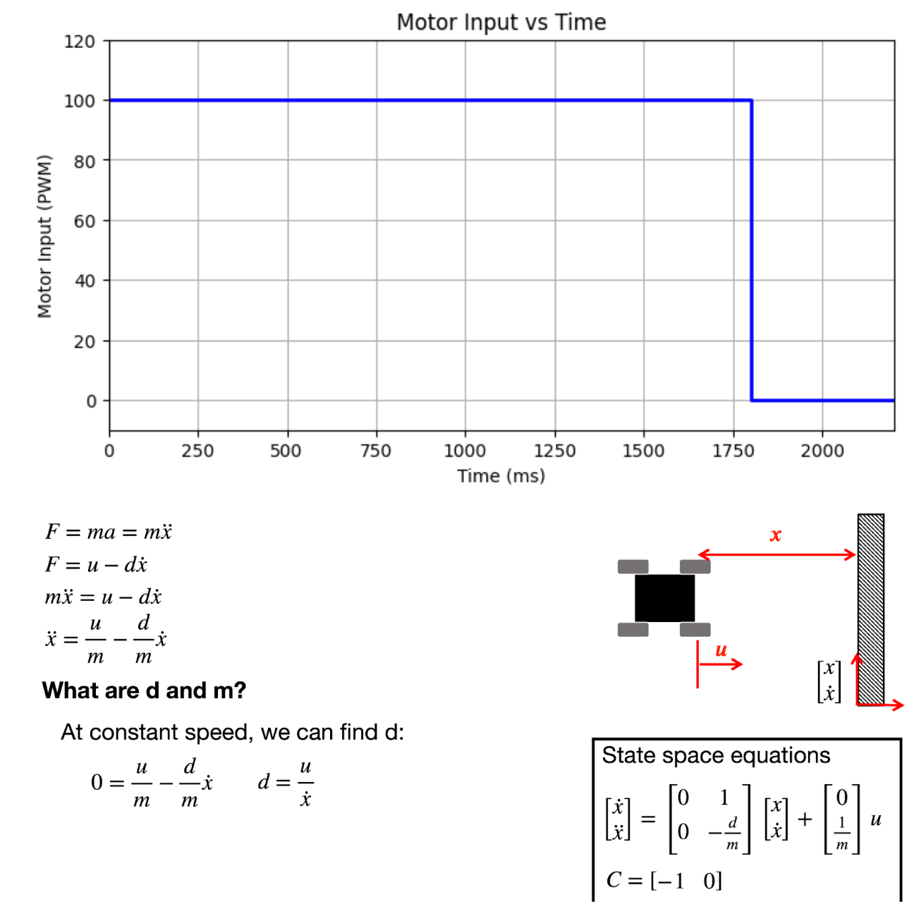
Distance=velocity*time so I set the robot to different constant PWM/velocities for the same amount of time open loop. I then observed the distance. Since time is constant, more velocity means more distance. I increased the PWM until I got a constant distance, meaning there is a max PWM where velocity no longer increases. I experimentally found this value to be PWM=200. I choose my step response to be 200*0.5=100.
To avoid damaging my car, I placed foam on the wall, then drove straight at 100 PWM for 1.8 seconds before braking. I started roughly 3 meters away from the wall.
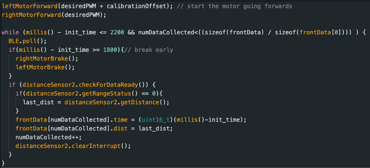
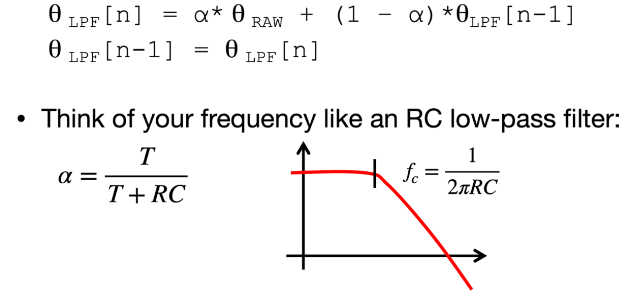
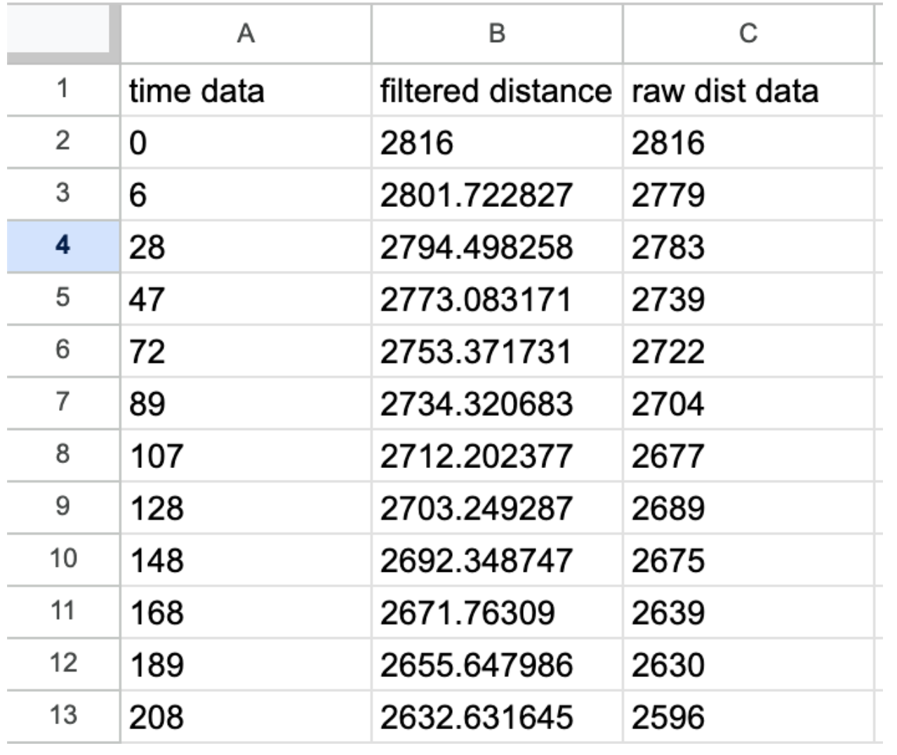
I first collected all the distance data. Then, I sent that data to the Jupyter Lab via BLE. I passed the data through a low-pass filter. Noise is high frequency, and the data is low frequency, so I want to essentially filter out the noise of my measurements. From the lecture slides below, I have T=50Hz for the frequency we collect TOF data and choose a cutoff frequency of 5Hz. The smoother/less noisy data results in more phase delay in the filtered data (trade-offs of choosing different cutoff frequencies).
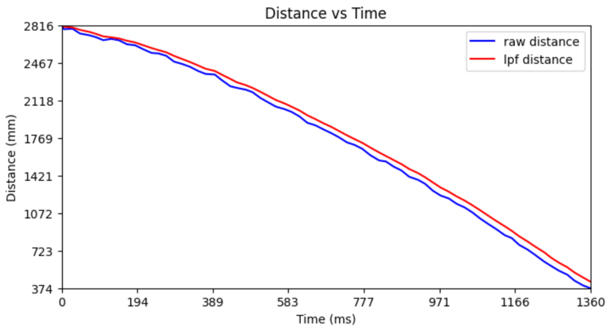
Plotted raw and lpf distance data starting from rest.
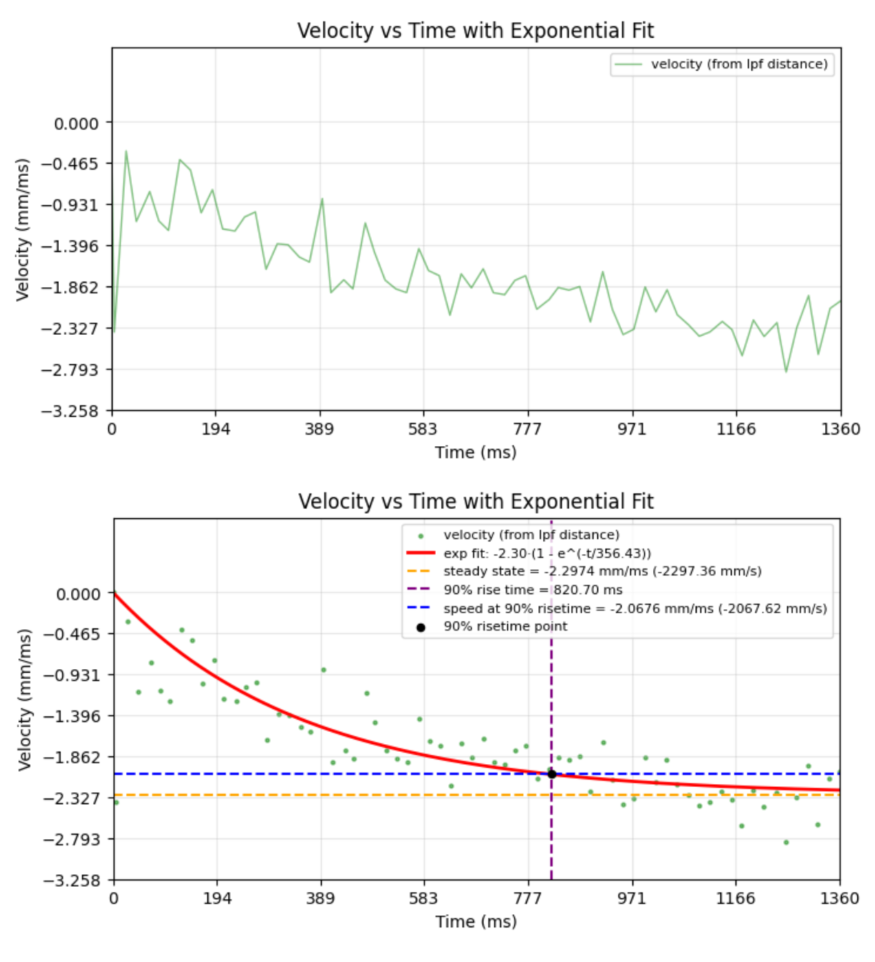
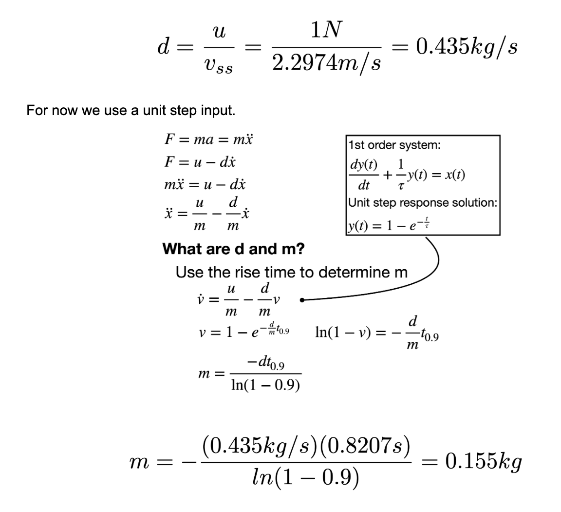
Then I used curve_fit from scipy.optimize to fit an exponential to the numerically differentiated lpf distance data. I then used the fit equation to find the v_steady_state. I got speed at 90% rise time from v_steady_state*0.9 and the 90% rise time from -tau*np.log(1-0.9) where tau is from the exponential fit -A*(1-np.exp(-t/tau)).
I then saved all this data in a CSV file.
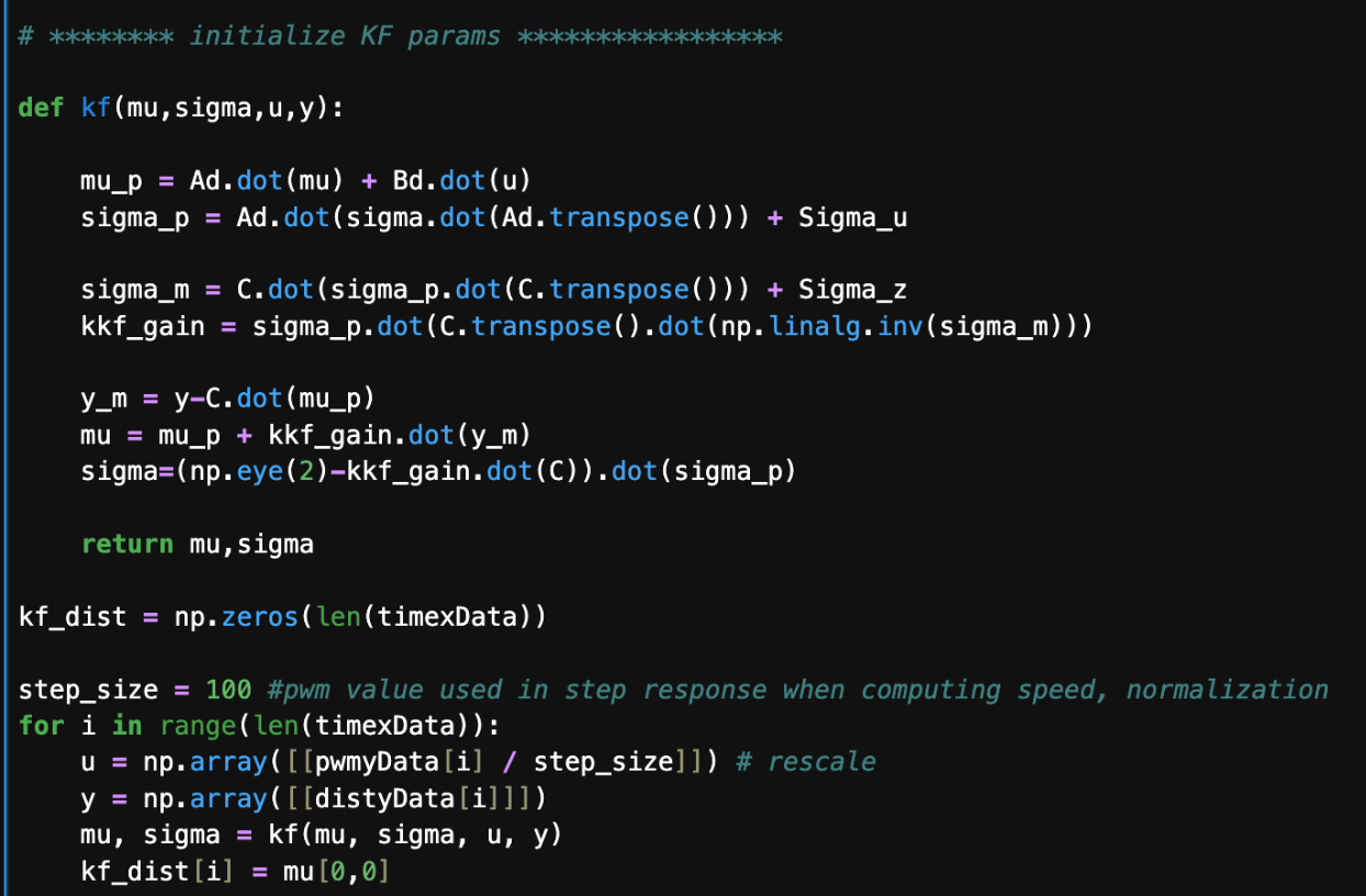
Initialize KF (Python)
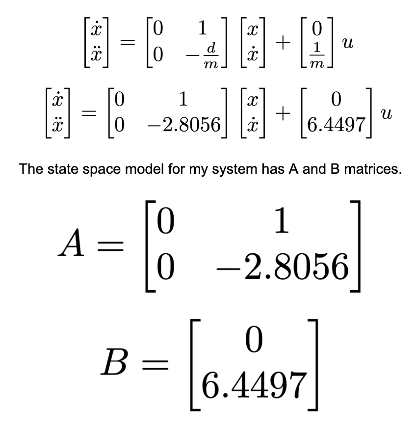
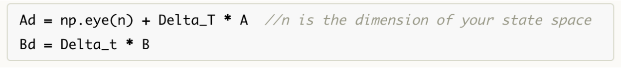
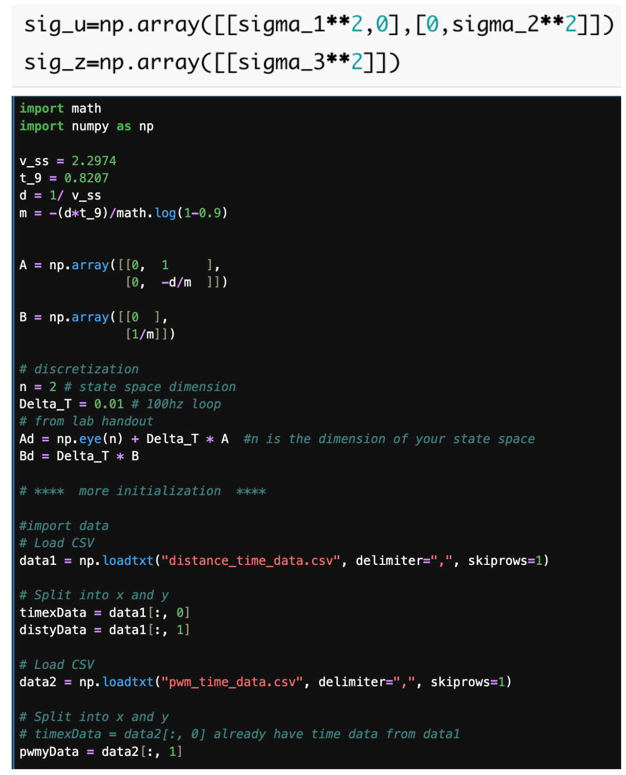
My sampling time from lab 5 was 0.008166s, but I chose a slower sampling time of 0.01s to be safe. Delta_T=0.01s is used to discretize my A and B matrices.
I define C=[1 0] since I sample TOF data as positive distance from the wall where the distance decreases as I get closer to the wall. This means my state vector x will initially be the initial positive TOF reading on the top and 0 on the bottom as we start from rest. x=np.array([[TOF[0]],[0]]).
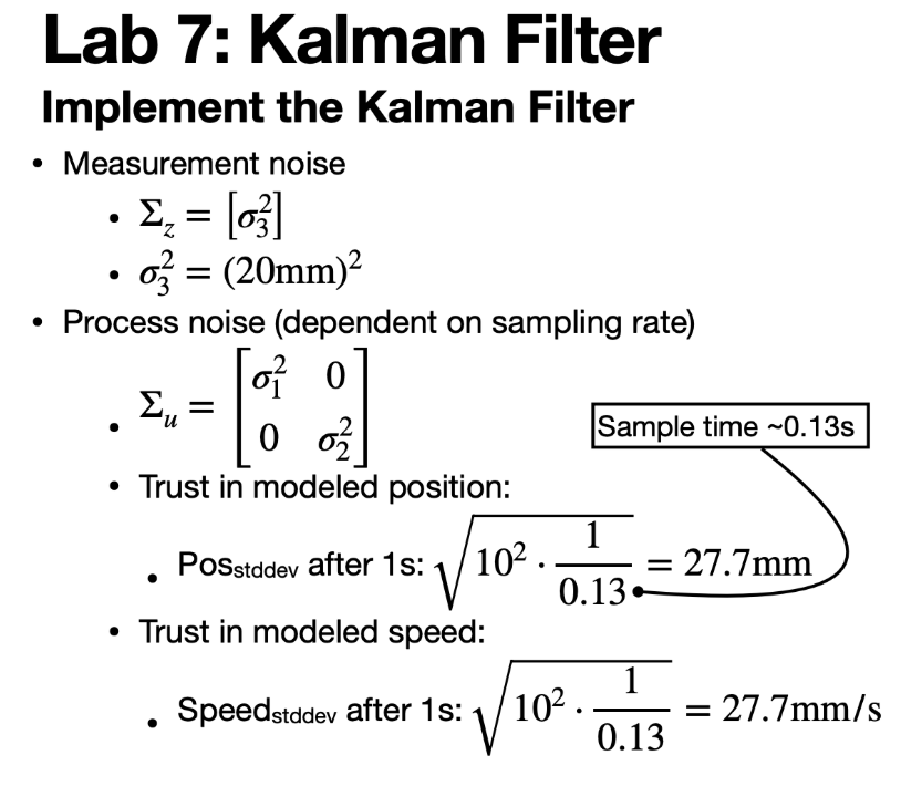
I now must make initial guesses for process and sensor noise covariance matrices. My measurement noise σ3 is initialized as the std of my TOF sensor. I placed the robot infront of a wall and kept it stationary and found the std to be 6.797178702320482 so σ3=6.8 initally. With a sample time of 0.01s I had initial guess of σ1=σ2=sqrt(10**2/0.01)=100. It is a balancing act of how much you trust your sensors and model.
Python Simulation
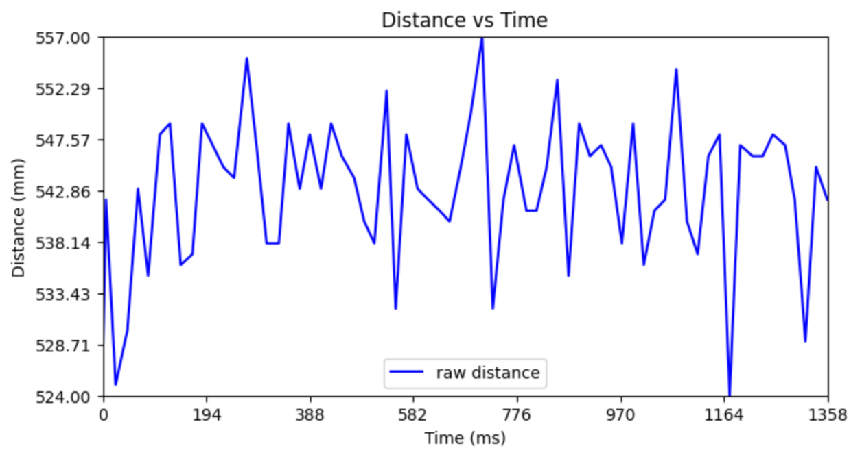
To practice tuning the covariance matricies, I simulate in Python first. I first imported TOF, timing, and PWM data from Lab 5 from a CSV file graphed below.
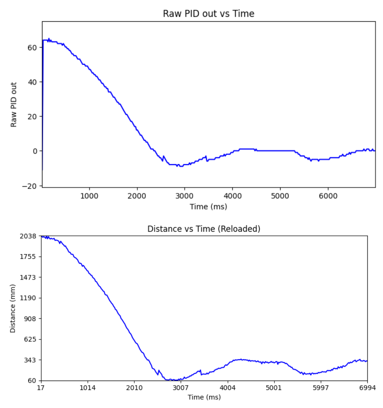
Since I already linearly interpolated in lab 5, my TOF and PWM array sizes are the same.
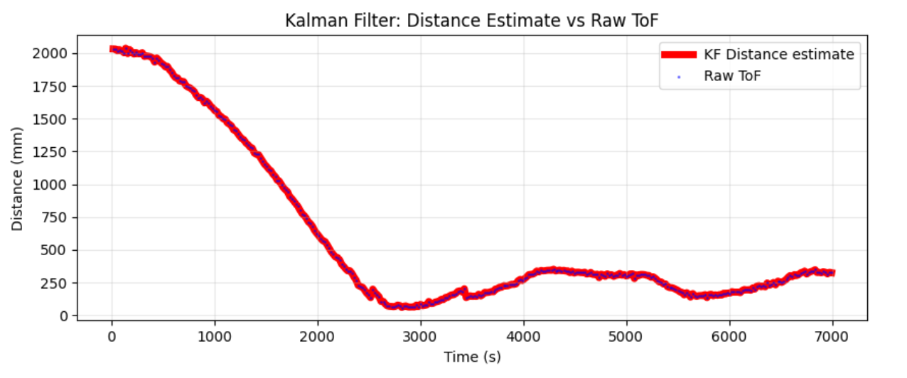
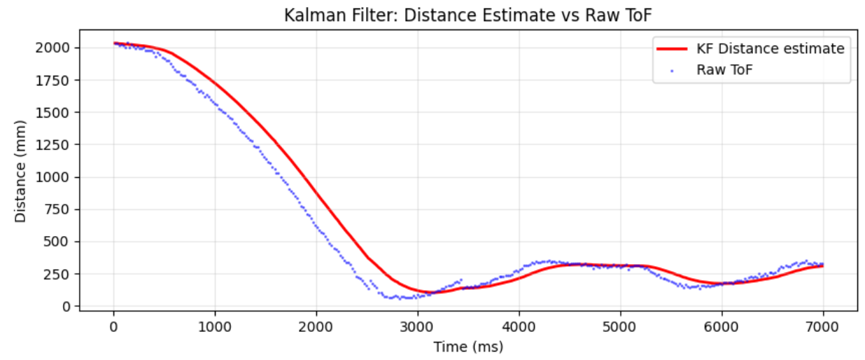
Graphed below is the initial guess of sigma1=sigma2=100 and sigma3=6. The KF tracks the TOF data too closely so we will have to tune further.
Model parameters affect my filter performance because if my calculated momentum or drag coefficients are off, then my model is less accurate. The covariance matrices affect how much I trust my sensor data and model. Sigma1 and sigma2 control how much I trust my model. Raising these values will mean I trust the model less and vice versa. The same goes for sigma3, where it is how much I trust my sensor measurements. If sigma3>>sigma₁=sigma₂, then I trust the model more than the sensor, which causes the filter to drift but be smoother. If σ3<<σ1=σ2, then I trust the sensor more than the model, and the KF will follow the TOF data closer but be more noisy. I can also have sigma1 and 2 be different values depending on how much I trust the modeled position and speed.
My initial sigma will affect how fast/slow I converge in the beginning. My Delta_T controls if I discretize the matrices properly, which can affect my performance. There are also different external noises that my model may not capture, which also affects my performance.
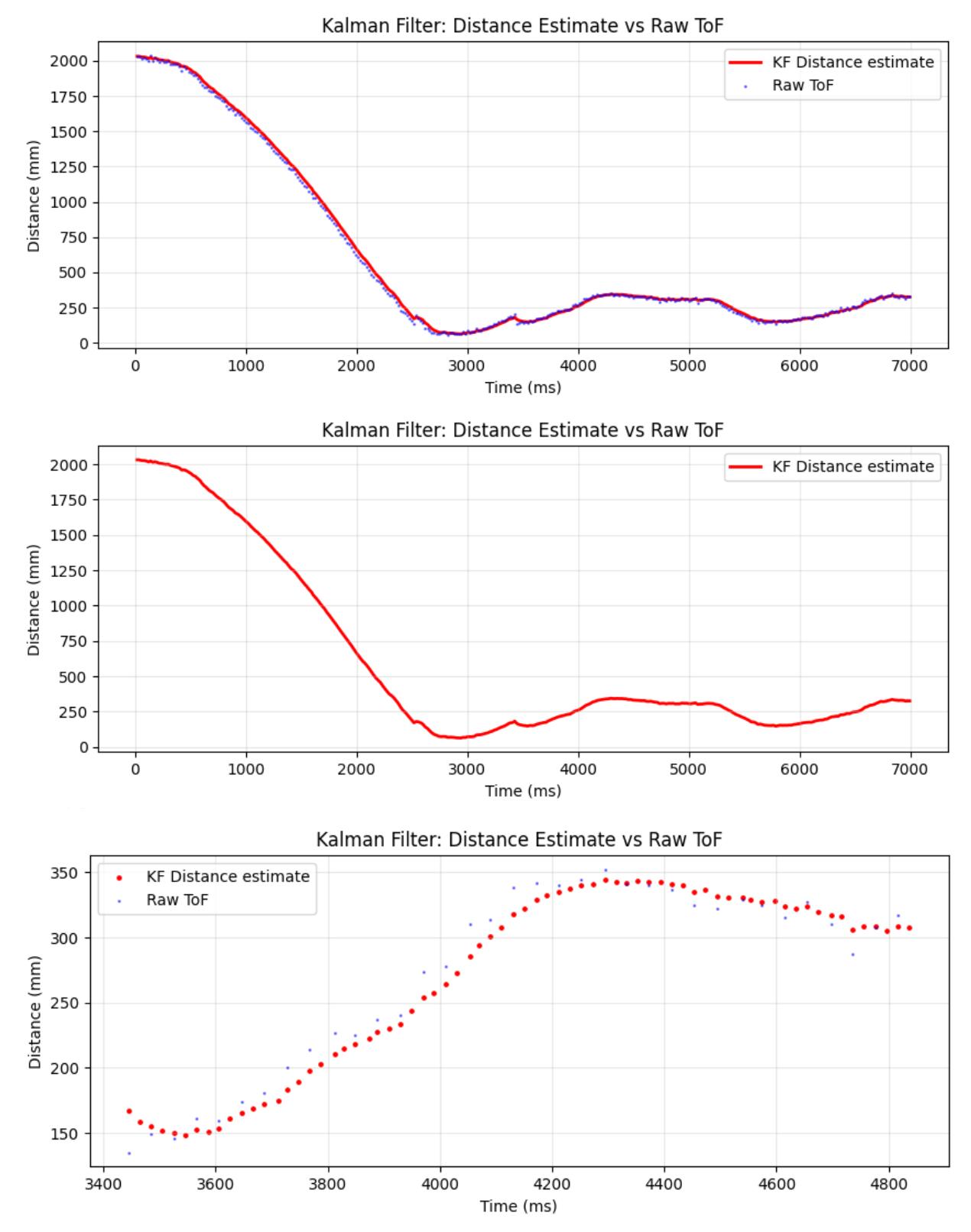
I first decrease sigma1 and 2 and increase sigma3 to trust the model more than the sensor and get the result:
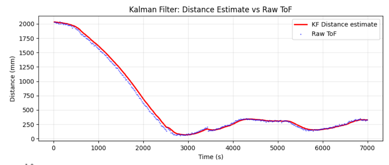
I decreased sigma1=sigma2=3 to trust the model even more and get a smoother curve for KF but now it is lagging.
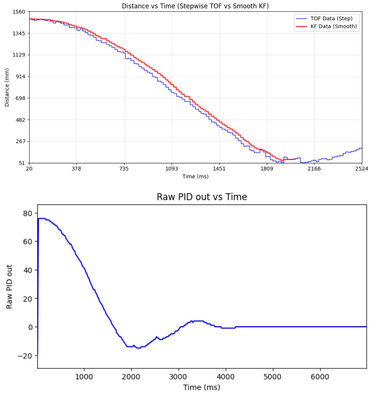
I kept tuning to get the final result below with sigma1=sigma2=8 and sigma3=20.
Robot KF Implemention
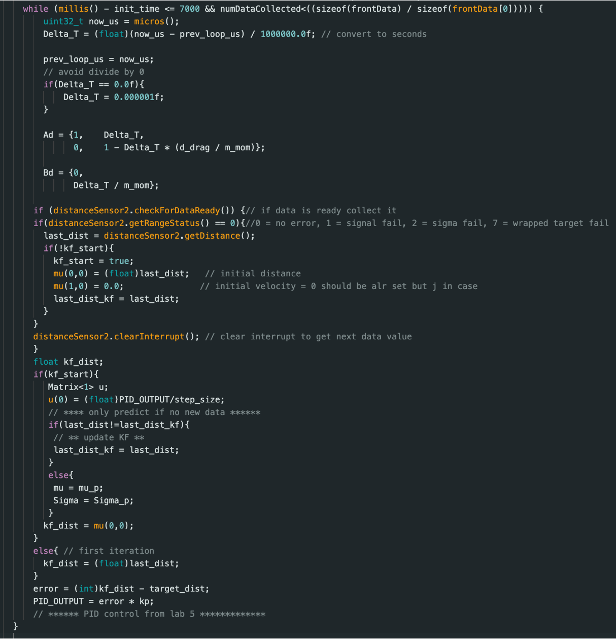
I now made the KF work in Arduino. BasicLinearAlgebra.h library is used for matrix math. Inspired by Aidan Derocher, I update the Delta_T value every loop iteration to dynamically recalculate Ad and Bd. My KF collects around 2000 data points, while the TOF sensor collects around 125 data points. I believe I could drive the robot even faster if I had a D term to slow down my robot as it got closer to the wall.
I first disconnect my motor battery to test hand movement in front of the TOF sensor to tune my covariance matrices.
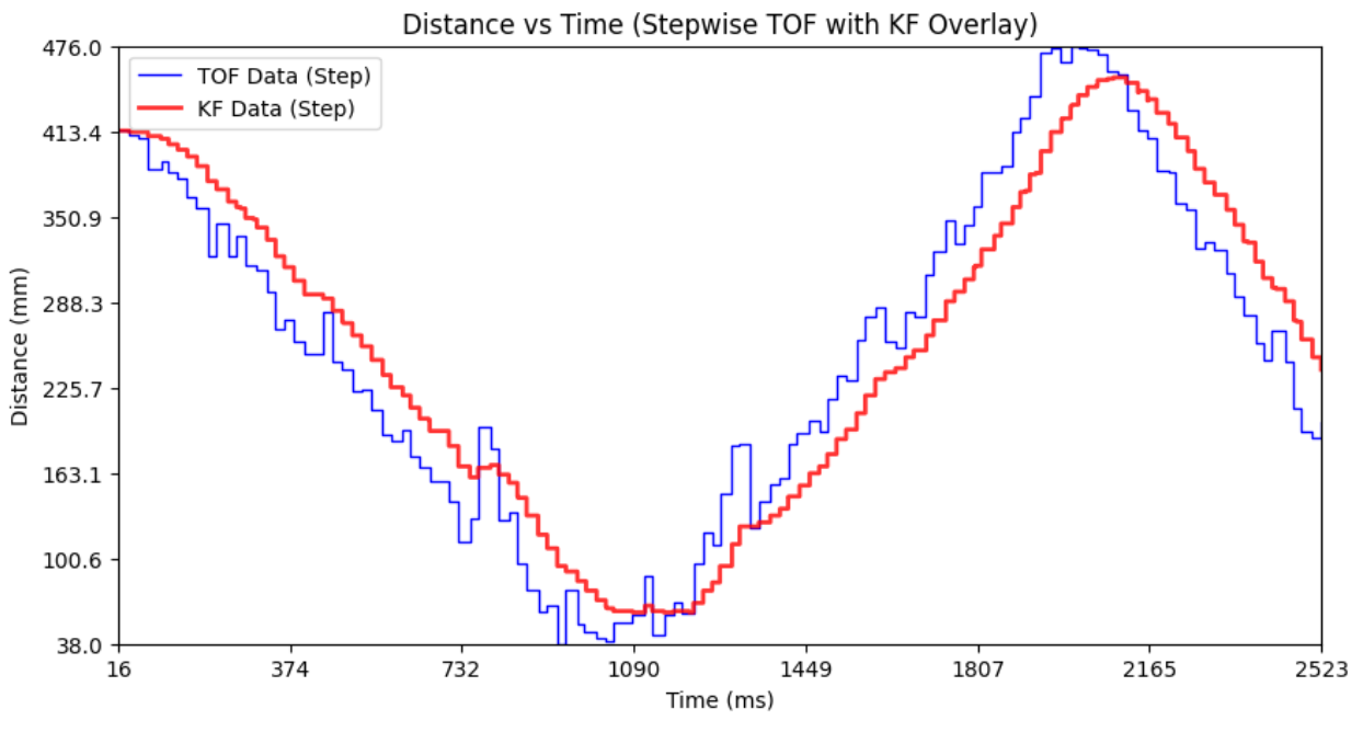
I then run the robot towards the wall with Kp=0.065, sigma1=5,sigma2=60 and sigma3=0.3.
Collaborations
Thank you Prof. Helbling. I referenced Jack Long’s and Aidan Derocher's webpages. Hunter inspired this website template. Claude was used to learn how the curve-fit python library works.