Prelab: Setup the IMU
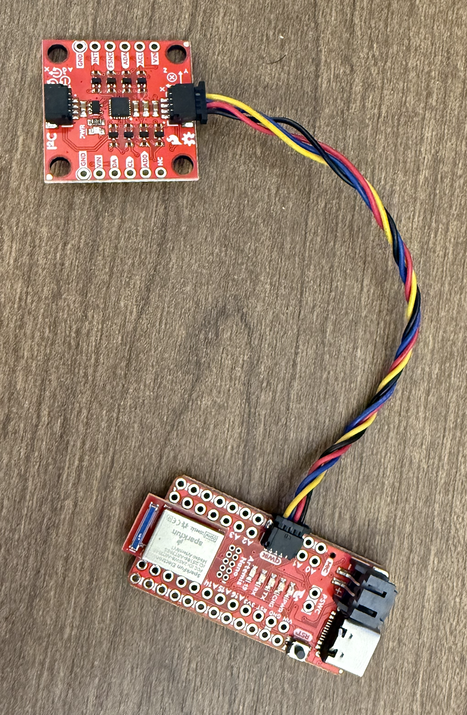
As prelab for lab 2, I set up the IMU by installing the “SparkFun 9DOF IMU Breakout_ICM 20948_Arduino Library” using the library manager. I then used SparkFun’s QWIIC connectors to connect the MCU to the IMU. A QWIIC connector is a 4-pin JST connector used for I2C devices so you can easily plug and play with different sensors.
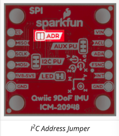
All I2C devices have a 7-bit slave address. According to the datasheet, our sensor, the ICM-20948, has a slave address of b110100X. The reason the LSB is X is because it can be either 0 or 1, and the AD0 pin determines this LSB. We want two different values for the LSB to differentiate between two ICM-20948 sensors on the same I2C line/bus. When the AD0 pin is logically high, then X=1, and when the AD0 pin is logically low, then X=0. Looking at SparkFun’s website, the default slave address of the sensor is 0x69=0b01101001, so here X=1, and thus AD0_VAL should be 1. If you wanted another IMU on the same line, you would have to solder close the ADR jumper on the back of the board, and then for that AD0_VAL would be 0.
I ran the Example1_Basics from the IMU library I downloaded and observed the sensor values as I flipped, rotated, and applied forces on the board so that it accelerated. For the acceleration data, you can see the acceleration in the xyz direction with units of mg (so divide the values by 1000 to get 1g=9.81m/s²). As an example, when the IMU is flat on the table with the Z axis of the IMU pointing out of the table, you can see that the acceleration in the Z direction is around 1020 mg=1.02g, which is a little off from Earth’s gravity of 1g=9.81 m/s². For the gyro data, this is the data in the xyz direction of the angular velocity in deg/second. When you don’t touch the IMU, it remains at close to 0 deg/sec in all directions, but when you start moving it, you can see the values changing in the direction of the axis that you move it. There is a video demo below.
I finally had the onboard LED blink 3 times slowly at the end of the setup routine so we know that the board is done setting up the IMU and Bluetooth even if we cannot see the serial monitor. You can see this in the video above.
Lab 2
Accelerometer
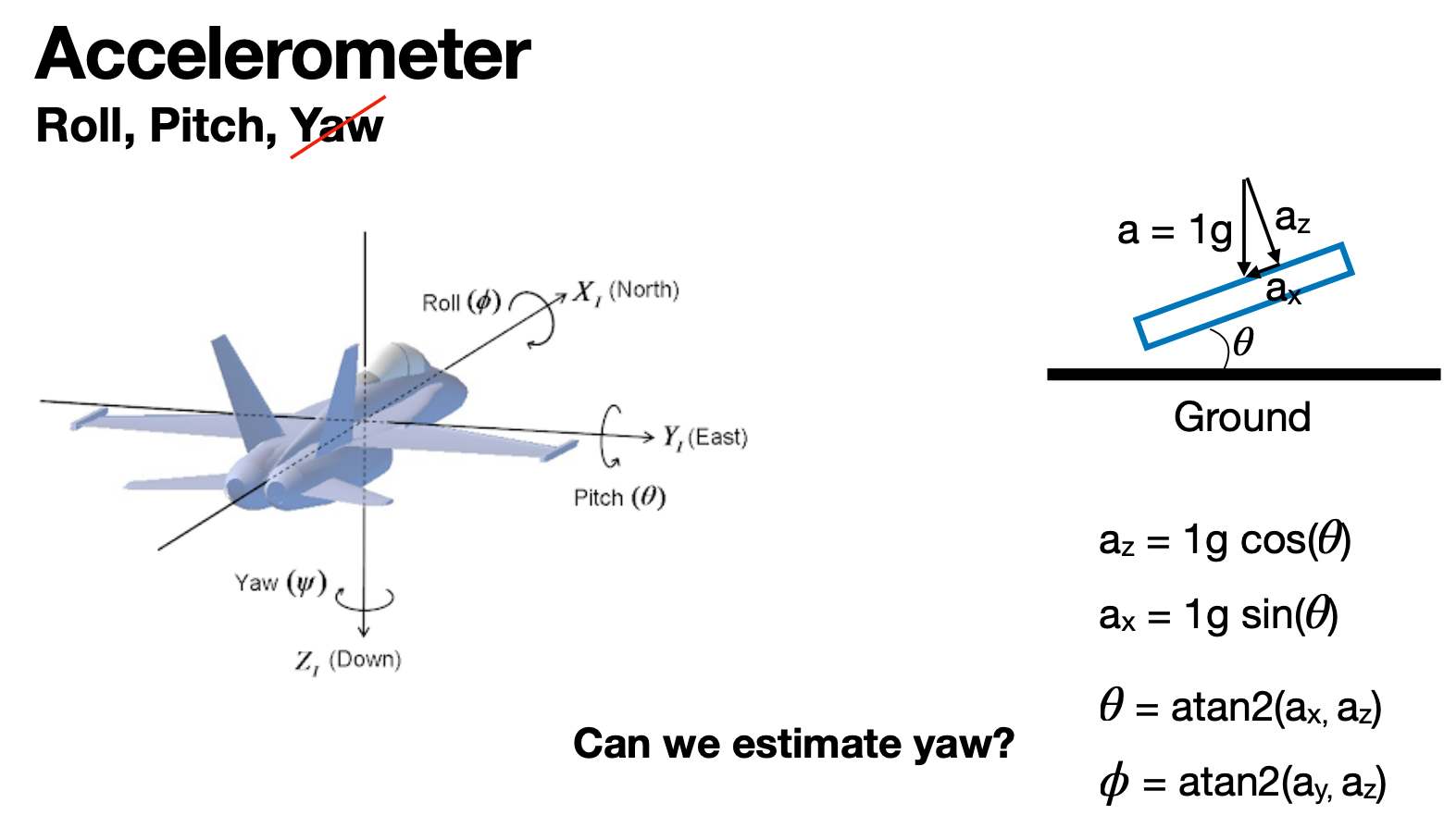
From class we found that pitch=atan2(ax,az) and roll=atan2(ay,az), as seen in the screenshot below. Our frame is flipped with z pointing up and y pointing west when the IMU is flat on the table facing up. So the only change is pitch=atan2(-ax,az). I created a helper function in Arduino to both print and collect the pitch and roll in degrees. I used the equation discussed above, which gives me the pitch and roll in radians from -pi to pi. Then I multiply this value by 180/M_PI, which converts the pitch and roll to degrees from -180 to 180 degrees.
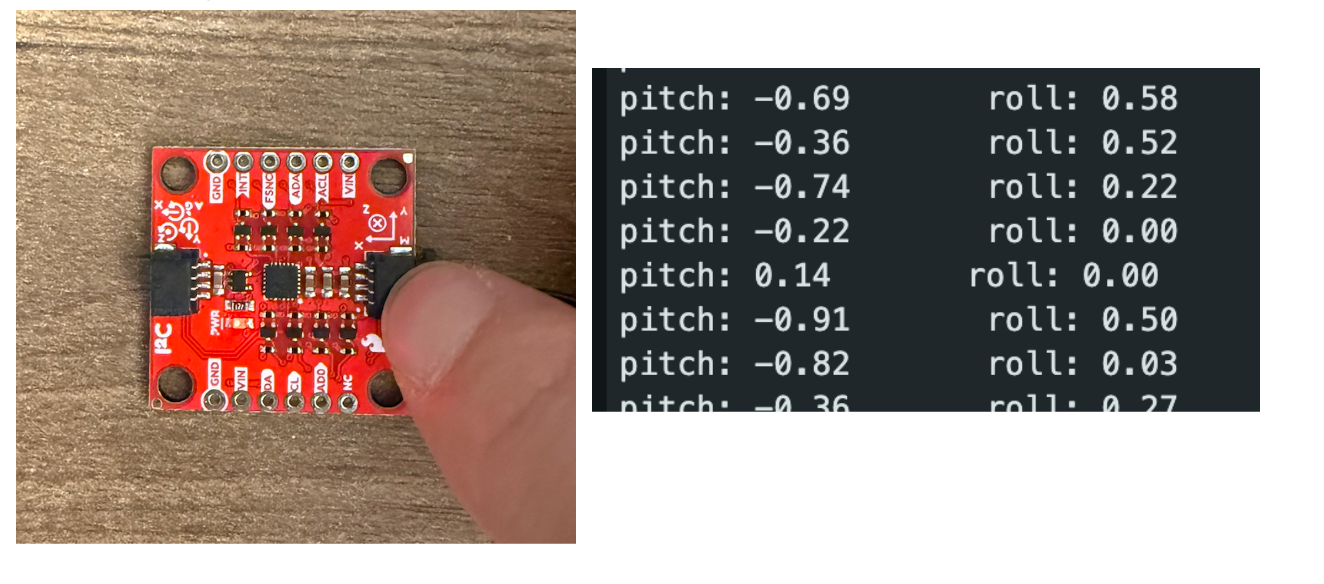
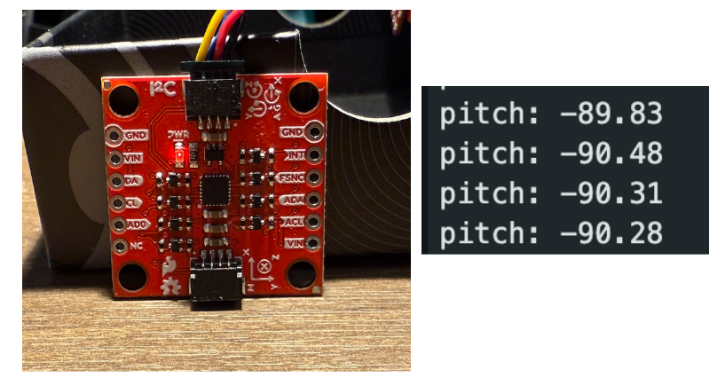
Below on the left is an image of the IMU flat on a flat table surface, so its roll and pitch should be 0 degrees, which they approximately are, as seen by the photo to the right (photo of serial monitor). Data is collected every second so that I have time to understand what the data looks like.
Below on the left is an image of the IMU oriented against a flat surface so we have a negative pitch. The right image shows around -90 degrees pitch.
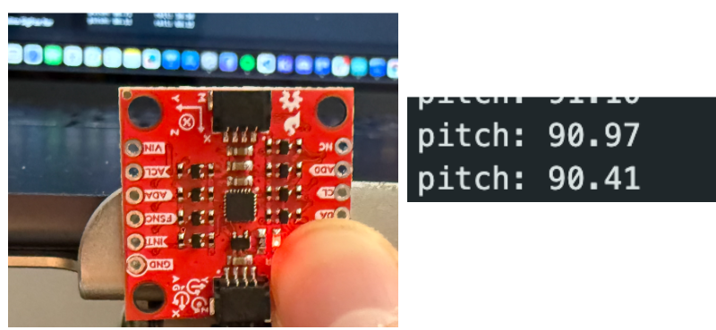
Below on the left is an image of the IMU oriented against a flat surface so we have a positive pitch. The right image shows around 90 degrees pitch.
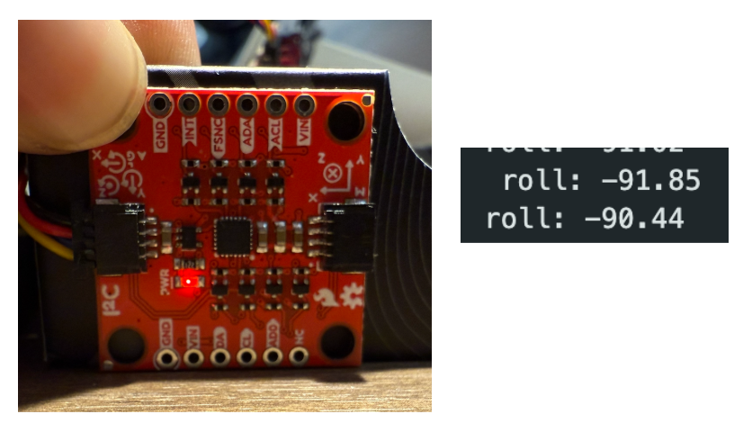
Below on the left is an image of the IMU oriented against a flat surface so we have a negative roll. The right image shows around -90 degrees roll.
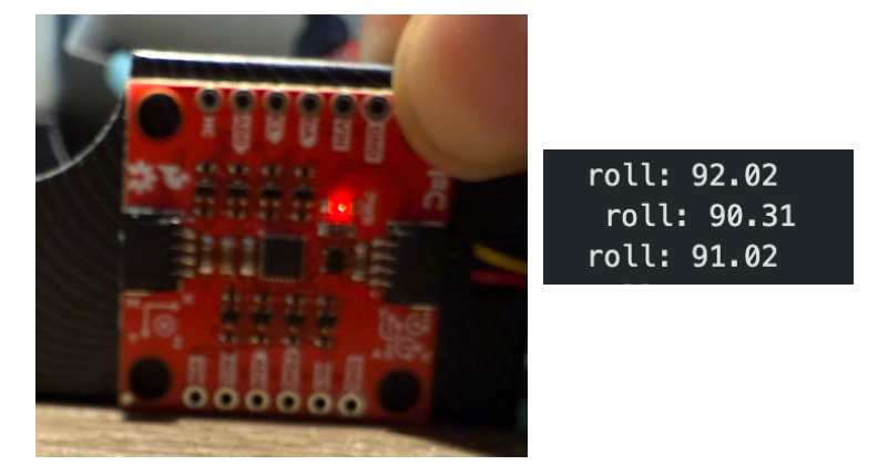
Below on the left is an image of the IMU oriented against a flat surface so we have a positive roll. The right image shows around 90 degrees roll.
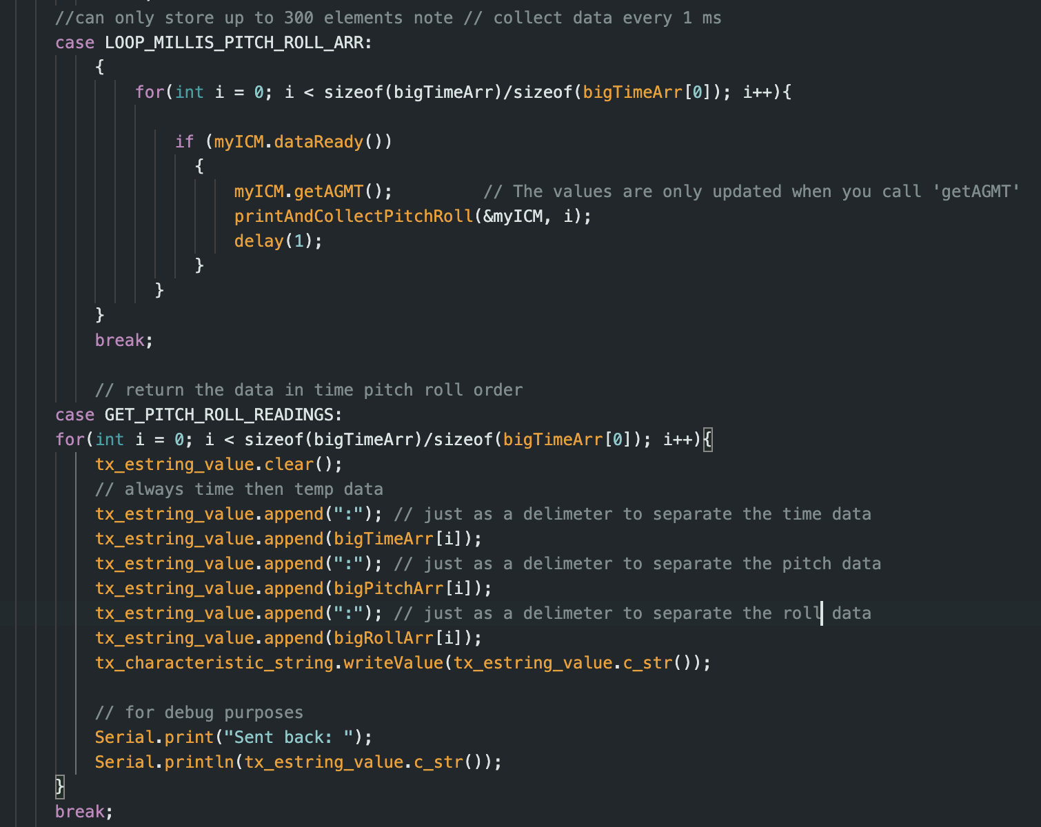
I also wrote two new commands similar to the get temperature and time commands in lab 1, where I save 500 data points of pitch and roll data with their timestamps in milliseconds. I called these commands in a Jupyter notebook and then plotted the data using matplotlib. I collect data every 1 ms, and the data is collected and stored in the global arrays in the printAndCollectPitchRoll(ICM_20948_I2C *sensor, int i) method. I will not show this method because it is trivial, and it just uses the sensor object to get the necessary data from the sensor, and the int i parameter is for what index we are going to store this new data in the global arrays. The Arduino scripts for the new commands are below.
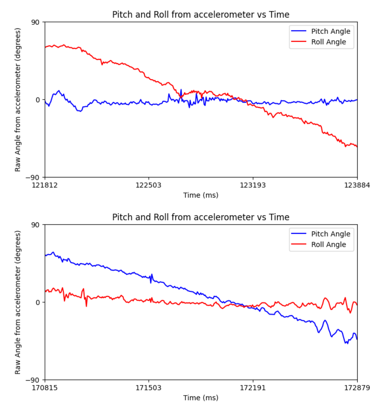
Below are two screenshots: the top one is where I rotated the IMU about its x-axis to see the roll change and the pitch stay constant, and the bottom graph is where I rotated the IMU about its y-axis to see the pitch change and the roll stay constant.
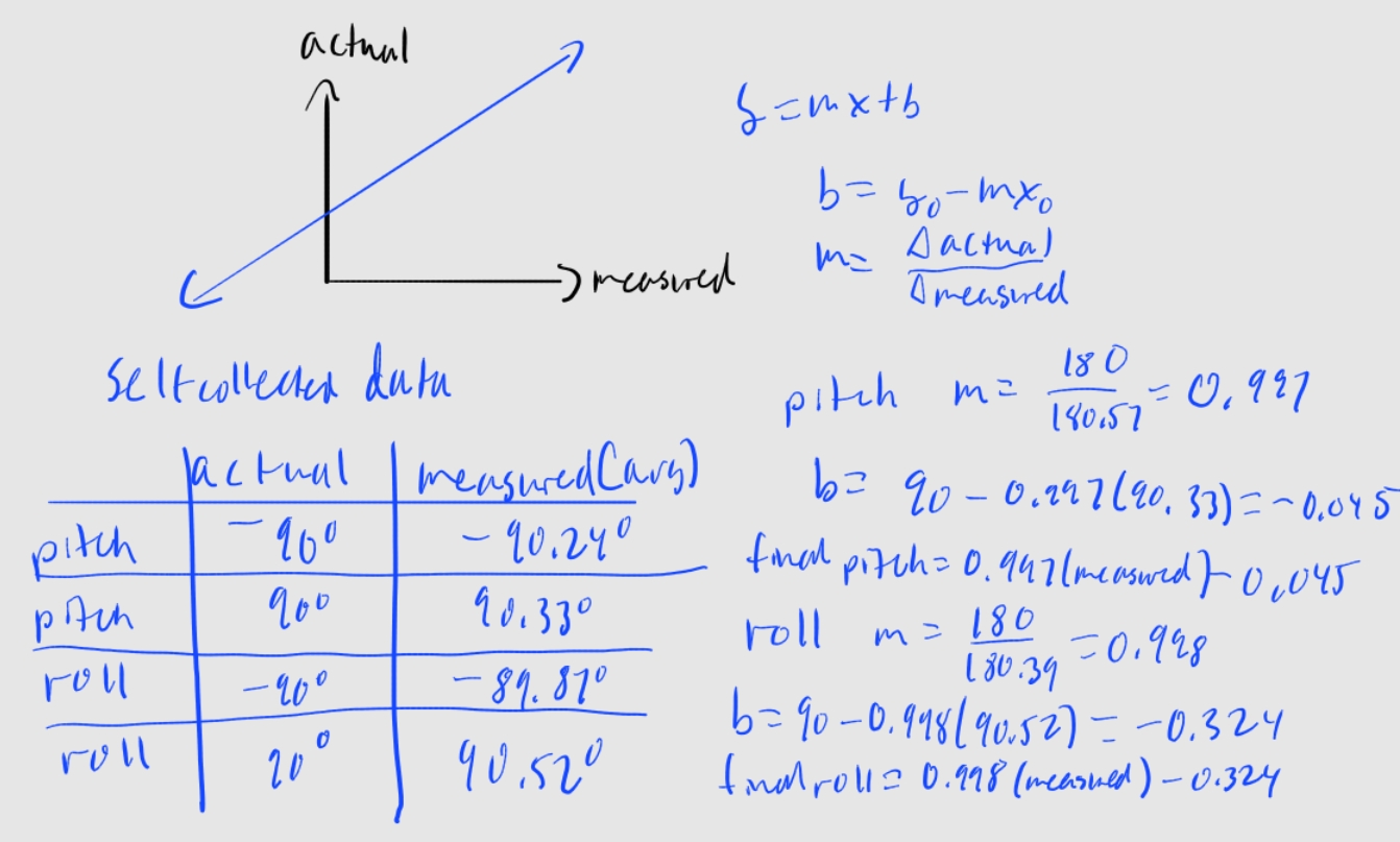
As seen in the screenshots above with the pitch and roll, my accelerometer is pretty accurate and only off by a couple tenths of a degree. Regardless, I still did two-point calibration as practice. I measured the average roll and pitch for what was supposed to be -90 and 90 degrees, as seen in the table below. Then, I calculated a conversion factor so expected/actual matches measured. The math is also shown below with the conversion factor I arrived at for roll and pitch. I applied these changes to my code, and it actually made my values less accurate. I was already so close to the actual value; I believe this two-point calibration is unnecessary for me.
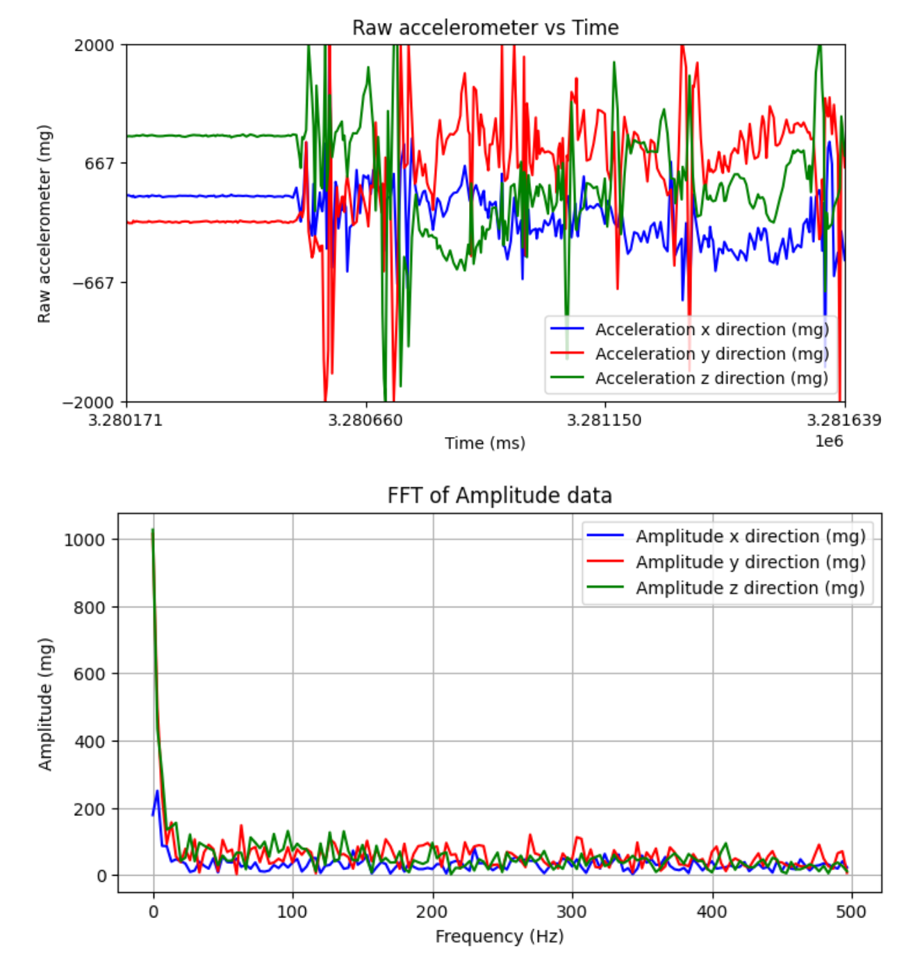
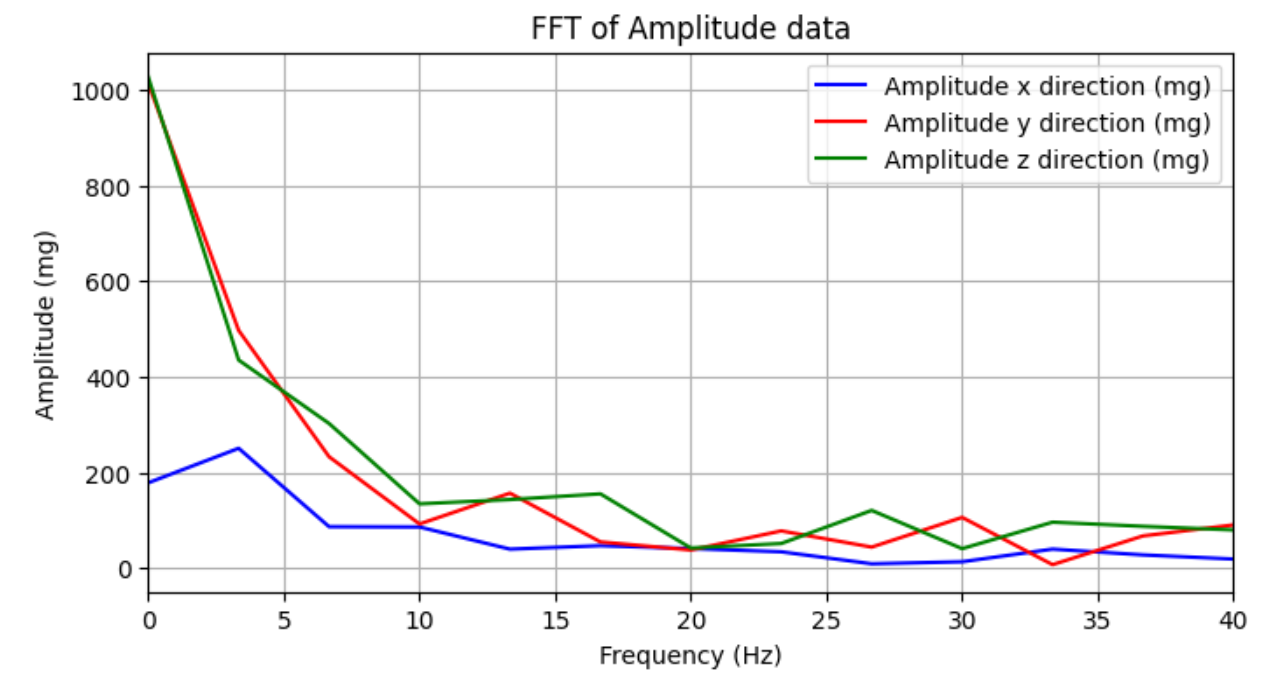
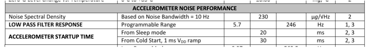
The accelerometer data is very noisy, as seen in both the time and frequency domains. All three graphs below use the same data from when moving the IMU around when it is next to a running RC car. A lot of the noise occurs at higher frequencies, as seen in the FFT, so I will use a low-pass filter with a cutoff frequency of around 7 Hz. From the FFT, the cutoff frequency is the frequency where the important, high amplitude, low-frequency data transitions to the high-frequency noisy data. fc=1/(2piRC)=7, so RC = 0.0227. From lecture alpha = T/(T+RC) and T=seconds/sample =0.3/300=0.001s since our trial lasted 0.3 seconds and we had 300 samples. So, alpha = 0.0421. A higher fc results in a lower RC, which results in a higher alpha. Conversely, a lower fc results in a lower alpha. The higher the alpha, the more you trust your raw accelerometer data and the less you trust your low-pass filter data. We have a pretty low fc, which is a low alpha, which means we trust our low-pass filter data much more than our raw accelerometer data, which makes sense. From the data sheet of the chip below, the noise spectral density is low at 230 ug/sqrt(Hz); for a small bandwidth of frequencies, the noise is small.
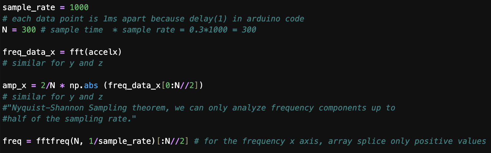
Below is the general structure of my code for how I achieved the FFT graphs following the tutorial from the course webpage.
Now, I (gently) bang my table (not out of anger but for experimental reasons), and the vibrations cause noise in the data. I also have the RC car running again. You can see the data in the time-frequency domain, and the data is much less noisy. You can see both the original (OG) signal and the low-pass filtered signal.
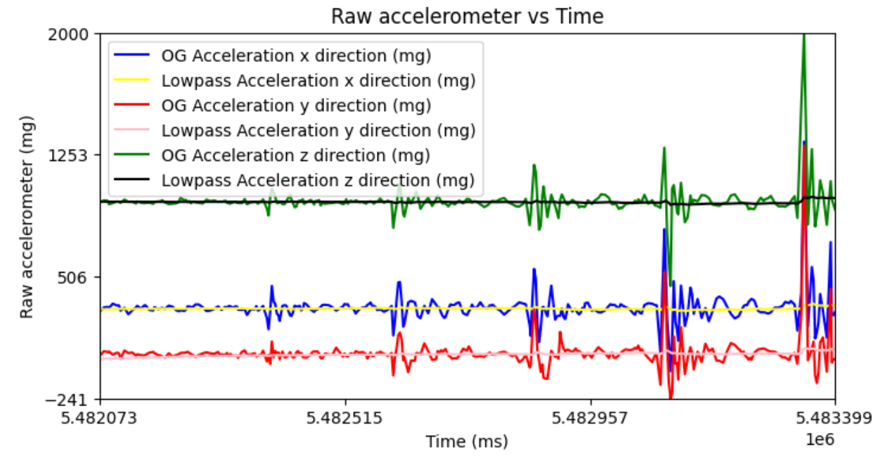
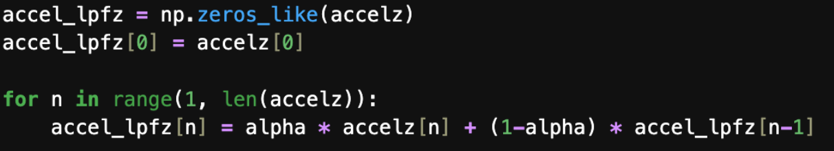
I used the data I already collected and low-passed it with my calculated alpha using the equation from the slides. Here is how I calculated the low pass for the z acceleration. Similar calculations for x and y acceleration.
Gyroscope
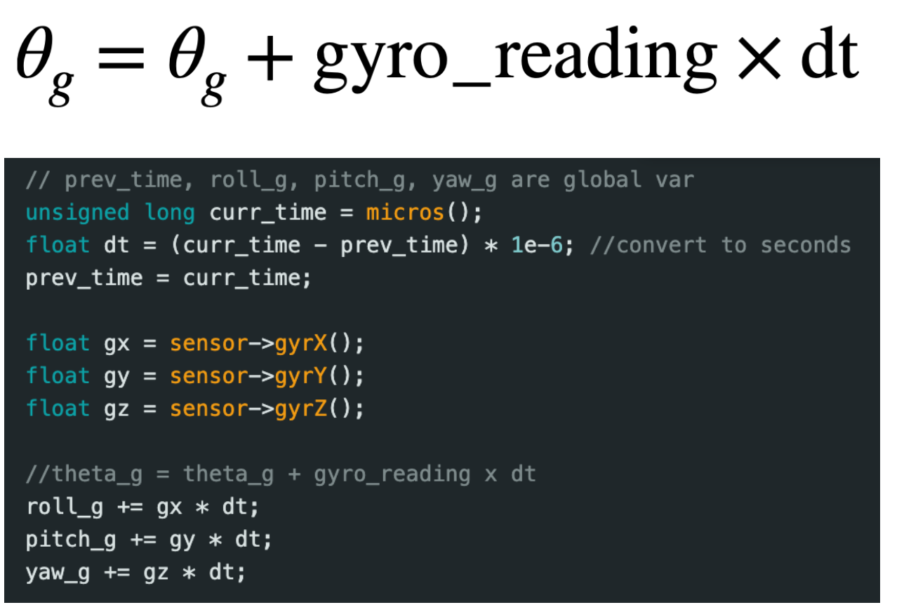
To compute pitch, roll, and yaw angles with the gyroscope data, I used the equations from class.
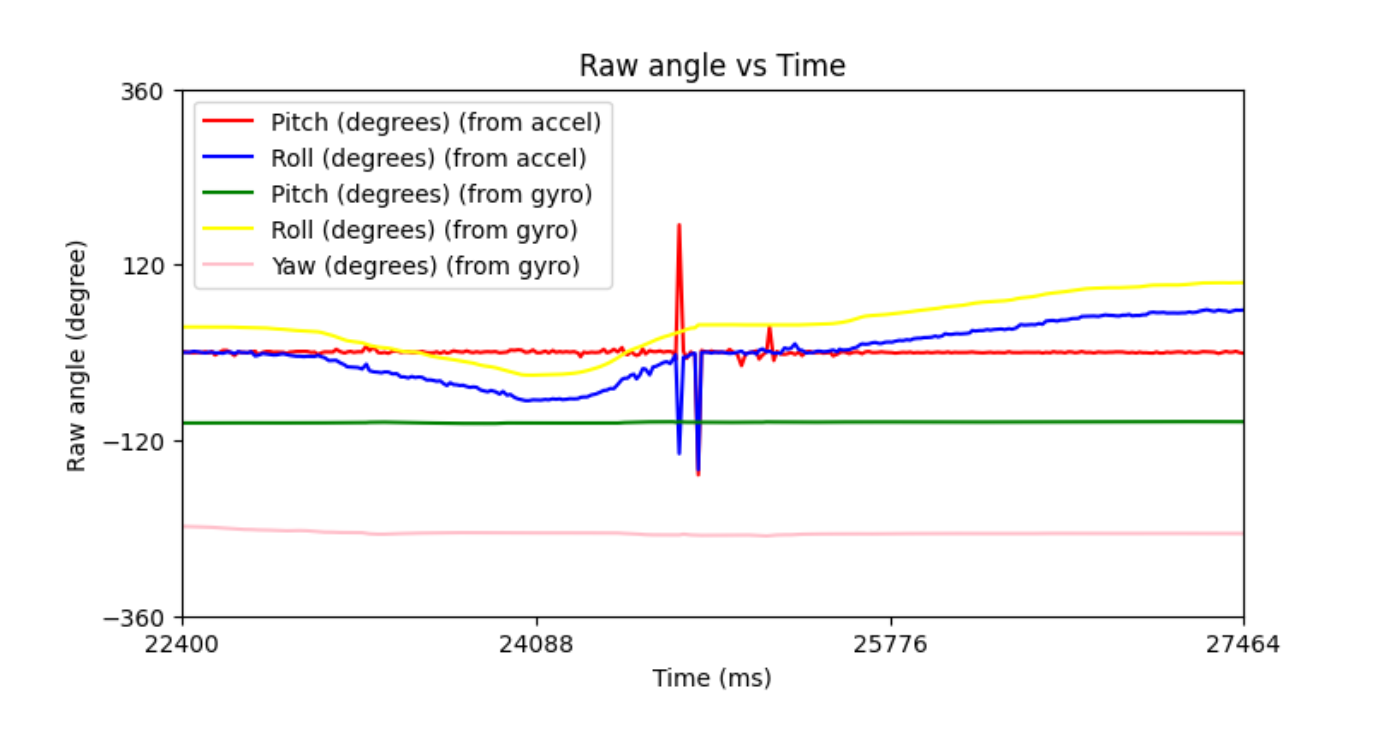
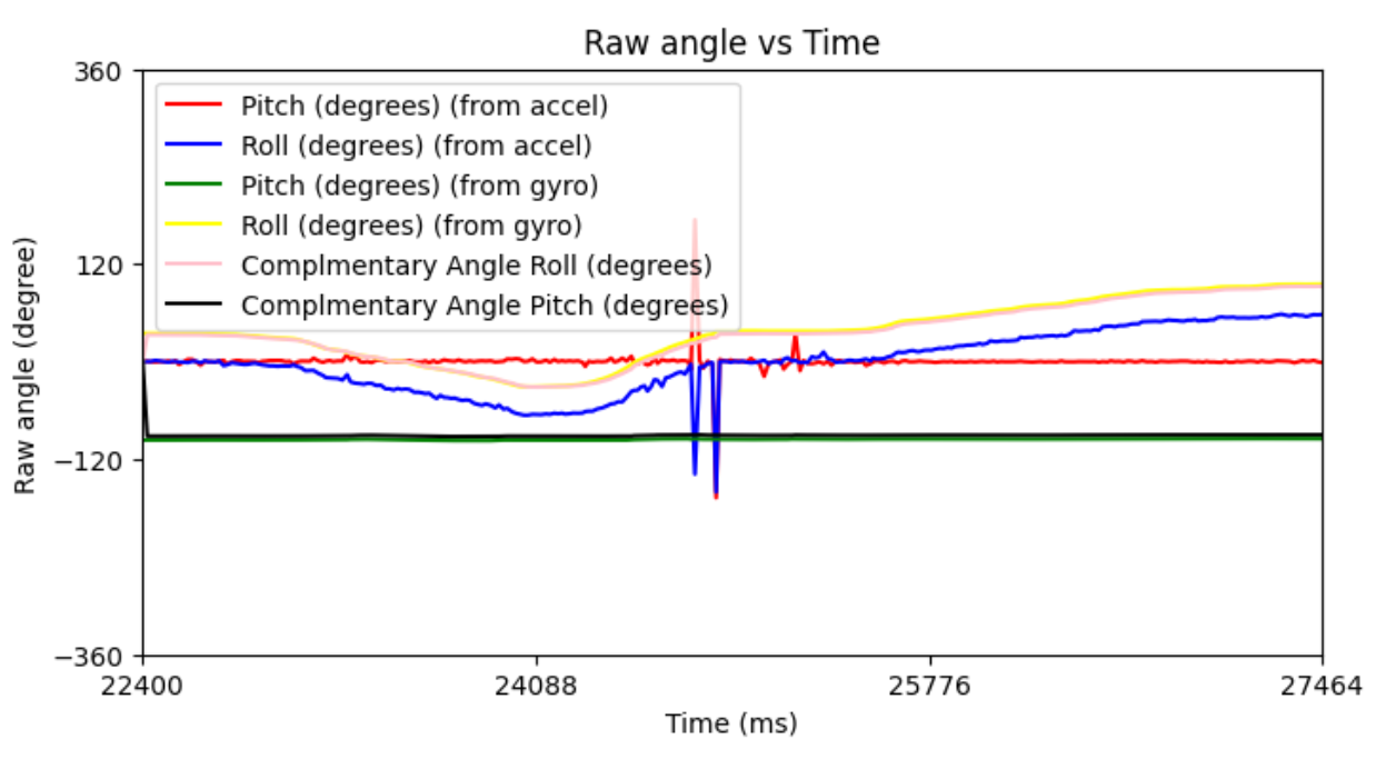
The unfiltered accelerometer data (seen in red and blue) is noisy, while the gyroscope outputs smooth, less noisy data (green, yellow, and pink), but it drifts over time, as seen in the graph below. By drift, I mean the values will climb in a certain direction due to accumulation of error. For example, 22400 ms have already elapsed since the start of the program, and you can see the gyro readings are already drifting away from the accelerometer-calculated angle. Errors will accumulate, and that's why our gyro drifts. We can’t really compare the yaw values since you cannot use the accelerometer to find yaw. If we adjust the sampling frequency and increase it, that would mean dt would be smaller, which means we would accumulate error in smaller magnitudes and thus have less drift, as I observed too. Less drift means more accuracy with our estimated angles with the gyroscope. It didn’t affect my accelerometer data. We are also working off of more gyroscope data. Now we can use a low-pass filter to deal with the accelerometer noise and a complementary filter to get the best of two worlds (the smoothness of the gyro and the non-drifting of the accelerometer).
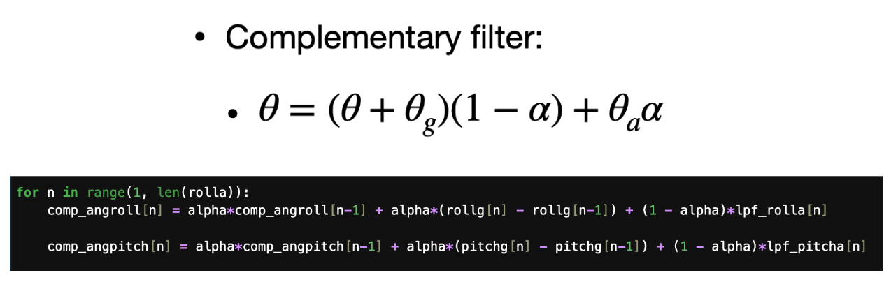
For the complementary filter, we trust the gyro for short periods of time (before it drifts and essentially high-passes) and trust the accelerometer for long periods of time (low-pass filter). Below I show a snippet of my complimentary filter code where comp_angroll and comp_angpitch are the arrays of complimentary angles for roll and pitch, respectively, and rollg and pitchg are the roll and pitch arrays that hold the angles calculated from the gyroscope. Lpf_rolla and lpf_pitcha are the low-passed acceleration-calculated roll and pitch angles, respectively. From the lecture notes, I chose an alpha of about 0.05 to high-pass the gyro and low-pass the accelerometer. The graph shows that I did this successfully because the pink and black lines follow the yellow and green lines well, which makes sense because this data was captured over a very short period of time, so we trust the gyro more for now.
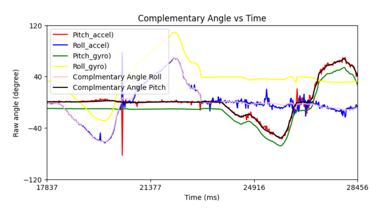
The graph below demonstrates the complementary filters' accuracy. As you can see, it closely follows the pitch and roll data from the accelerometer graph but is smooth like the gyro data. It is not susceptible to drift here because even though the gyro data drifts a lot, it still stays close to the real value, as seen by the 0 degrees of pitch and roll.
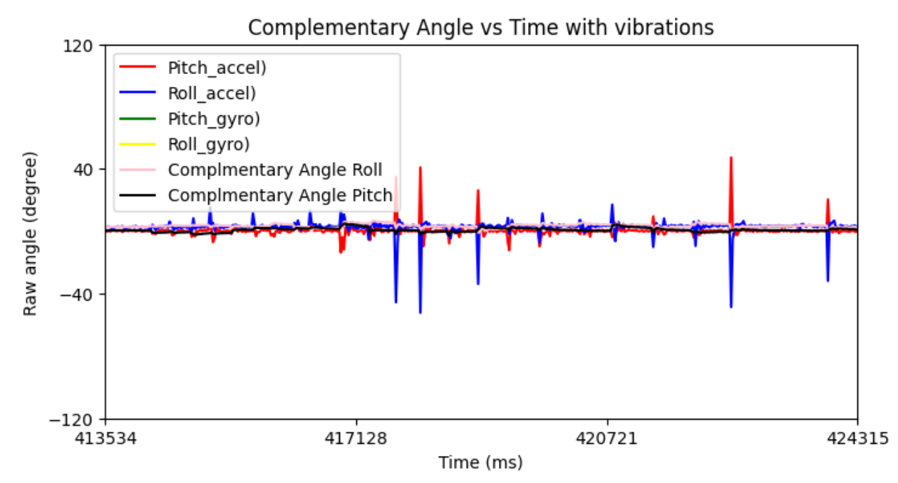
I vibrated my desk in the graph below and you can see how with the complementary filter, the IMU is not sensitive to vibrations.
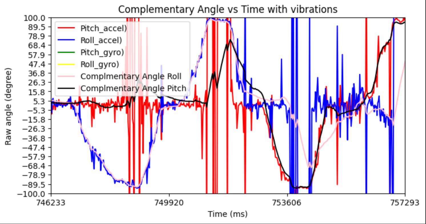
As seen by the graph below, the working range is around -90 to 90 degrees for both pitch and roll.
Sample Data
I no longer wait for IMU data (so remove the delays), and I just check to see if the data is ready. In my testing, 0 delay will still give me data every loop iteration. Still, I have this conditional check to see if the data is ready so we only save data that is ready (no programmed delay). I also removed other delays in my program and serial.print statements since those also slow down my program. The data went from 54973 to 56379 ms, and there are 500 data points, so (56379-54973)/500=2.812. So on average, it takes around 2.812 ms to collect one data point to the next data point collection, which gives a frequency of 354.61 Hz. My main loop on the MCU does not run faster than the IMU produces new values because I did not get a serial printout saying the data was not ready (before I commented out all prints). Also, I had a counter variable to see how many times the data wasn’t ready, and it returned 0. It is possible, though, that maybe my code is still not fast enough, and thus if I sped it up more and found more ways to get it to be faster, I could maybe run faster than the IMU produces values.
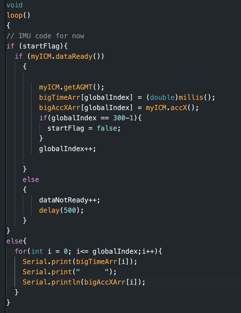
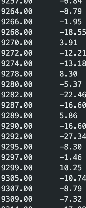
Like in Lab 1, I use the main loop to store IMU data (specifically x acceleration here) in arrays with the time stamp. I use flags (startFlag boolean) that, when the program starts, start recording the data, and when the array is full, stop recording the data and just keep printing out the collected values in the serial monitor. This boolean could easily be replaced with something like a button press so that you can control when you want to collect data.
To my knowledge, from a space and time complexity standpoint, there would be no difference. You still have the same amount of data, and whether you have two arrays or one 2D array should not affect the time complexity of loading and reading the whole array, and it should not affect the amount of space it takes on the MCU. I think just conceptually, though, we should have separate arrays for storing accelerometer and gyroscope data just because they deal with different quantities (mg and deg/s). You could also argue for the big 2D case because we are collecting the data at close to the same time, and we are fusing the sensor data, so we will have the same amount of data points. In my opinion, the best data type to store my data is a float. Floats are 4 bytes, which is less than a double, and integers also have 4 bytes but less granularity (no decimals). Strings are practically character arrays, and each character is 1 byte, so the longer the number, the more bytes we will have, which is not good. In another class, we used fixed-point arithmetic, which could be interesting to look into in the future, but it is not one of the options provided. As discussed in lab 1, this MCU has 384 kB of RAM. Since I am using floats, that is 4 bytes per entry, so 384 kB/4 B = 96000 array elements of floats, but we are also limited to memory for other stuff we need to store. But assuming we have 96,000 array elements and we want pitch and roll data from the accelerometer and gyroscope and the current time associated with it, that is 5 floats per instant of time we collect the data. So we really only have 96000/5=19200 sample points (and sample at around 2.8 ms/sample), so that would be 53.76 seconds of data.
500 data points gave me 1.406 seconds of data, so I’ll need around 1800 data points to give me over 5 seconds of data. I got 24321-19546=4775, which is a little under 5 seconds, so I ran the test again with 2000 data points since this doesn’t seem to scale exactly linearly. Now I have 34432-29075=5357 ms, which is 5.357 s, so this is at least 5 s of IMU data, which was also sent to the computer via Bluetooth. The data I recorded was pitch and roll from the accelerometer and pitch, roll, and yaw from the gyroscope.

Stunt!!!!
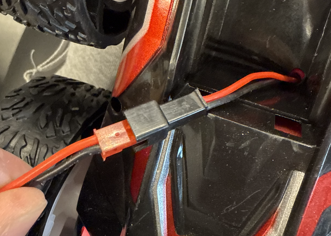
First, I made sure the battery was plugged in where the black wire was connected to the black wire and the red wire was connected to the red wire as seen below.
After playing with the car for a bit, the car goes really, really fast (much faster than I thought). It can make turns and go forwards and backwards quite fast. It also picks up speed fast (big acceleration). One trouble is that it is so fast that even small inputs in the remote control lead to big displacements, and it is hard to control over small displacements. The following videos below are some of the stuff that I tried. The robot can turn in place about its center of mass and can go forwards and backwards as well as flip on its back. It also has a mode where it completely tweaks out, as seen in the last video. If you go really fast one direction and immediately go the opposite direction it will flip. It kind of drifts when it turns in place but can drive in a straight line decently well for short distances.
Collaborations
I would like to thank Prof. Helbling and TA Julie for their help in lab and quick responses on ed. I referenced Aidan McNay's, Aidan Derocher's and Stephan Wagner's webpages from previous semesters. Generative AI was used in lab for helping understand the lab handout, refreshing on python syntax (especially when it comes to graphing), and helping code to this website. This website template was also inspired by Hunter. Hunter also helped me with my understanding of complementary filters.