Overview
I had the very ambitious goal of doing both lab 12 options. Unfortunately, my Bluetooth was buggy, so I did the inverted pendulum, where the robot is initially in its normal position and then drives very fast forwards, briefly brakes, drives backwards, and then initiates the controller mid-flip to maintain the balancing position. I don’t have any plots, as my Bluetooth was finicky.
Approach
I use the DMP as the process variable for the P and I terms and the raw gyroscope as the process variable for the D term. Then it was a matter of tuning the gains and applying other techniques like having a deadband and working on the flip to get everything to work together.
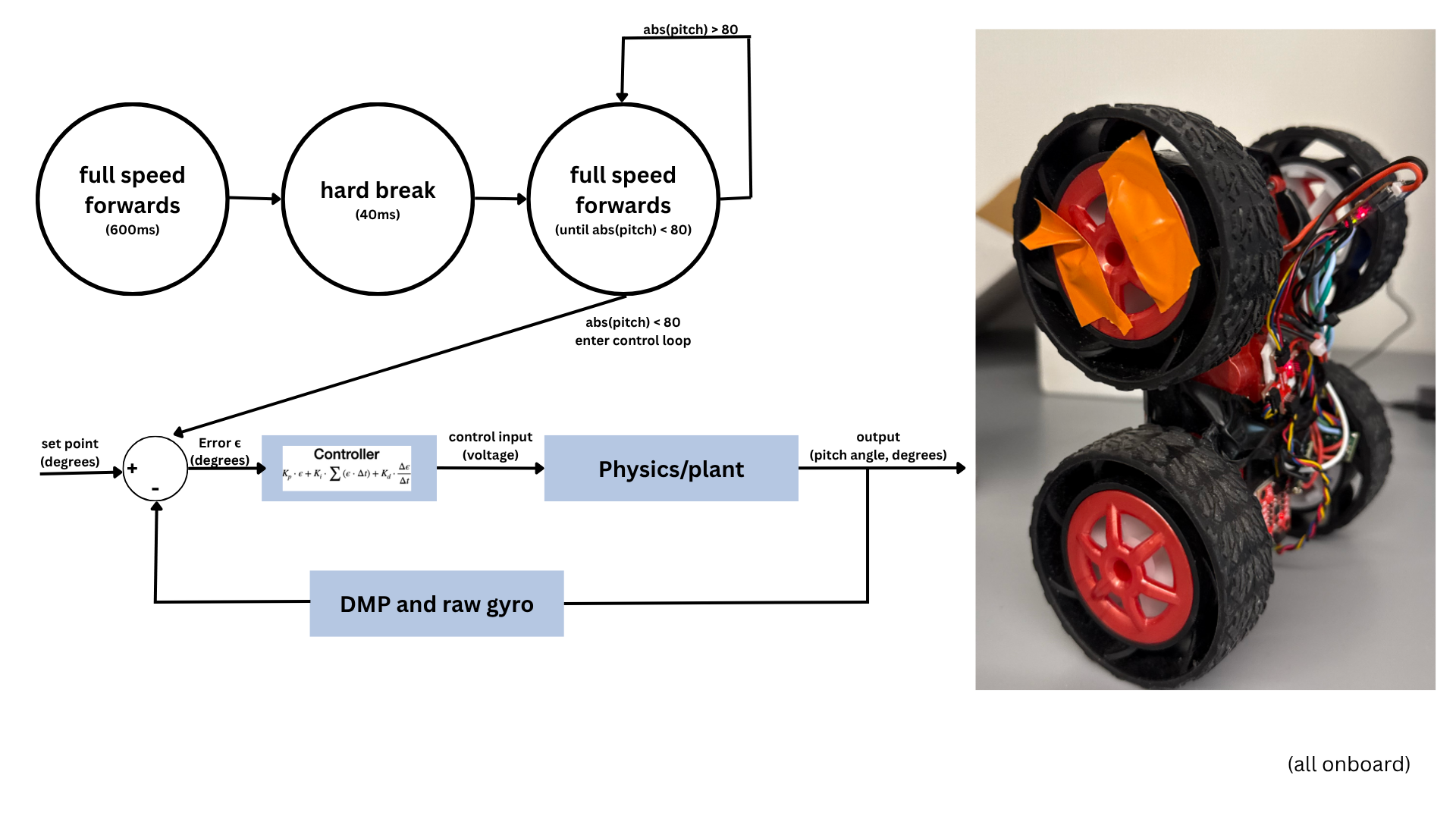
Figure 0. High-level diagram of my sequence for the wheelie.
Process Variables
The process variables need to be accurate since the set point will be some magnitude of tenths of a degree within 0° for the balance point. The process variables also have to update quickly enough, as if our control loop’s operating frequency is too low, we will not have enough time to “react” and self-right ourselves. Dimitri, an ASML engineer who gave advice on the inverted pendulum, suggested the control loop had to operate at least at 1 kHz to balance. I considered using a complementary filter, but from Lab 2, I only had a frequency of 354.61Hz.
The DMP gets accurate, non-noisy data with minimal drift but updates at 28.6 Hz. I use this process variable for the P and I terms of the controller. To compensate for the slow update time, I used raw gyro data for the D term. Since it measures angular velocity, I used this instead of taking the derivative of the error. The D term must update fast to catch the car if it tips over fast. With direct register reading, I get a frequency of 1.4 kHz.
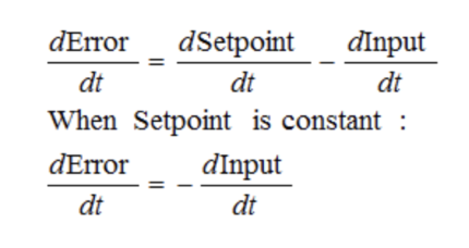
Figure 1. From Brett’s blog showing that the derivative on error is the negative derivative on measurement when the set point is constant.
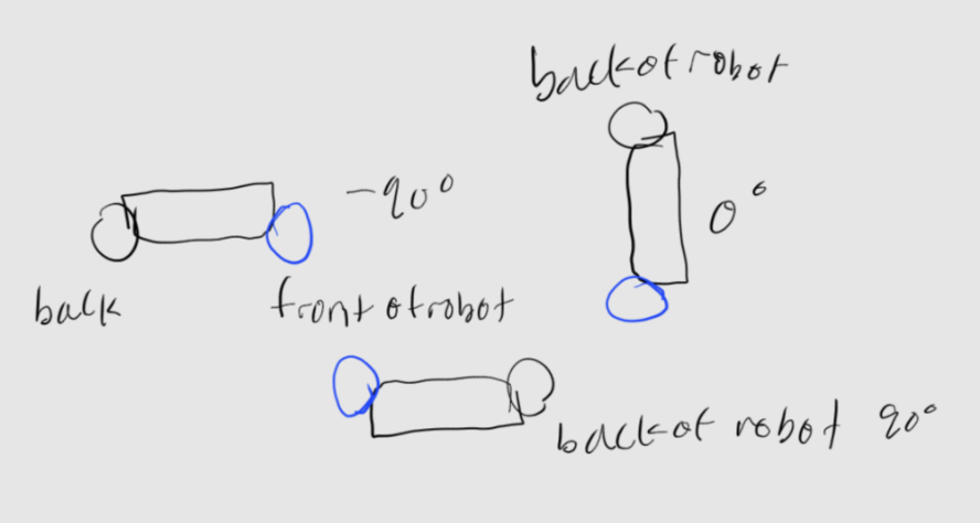
Figure 2. Relative pitch of the robot when it is flat on the ground (top left), when it is balancing upright (top right), and when it is upside down (bottom middle).
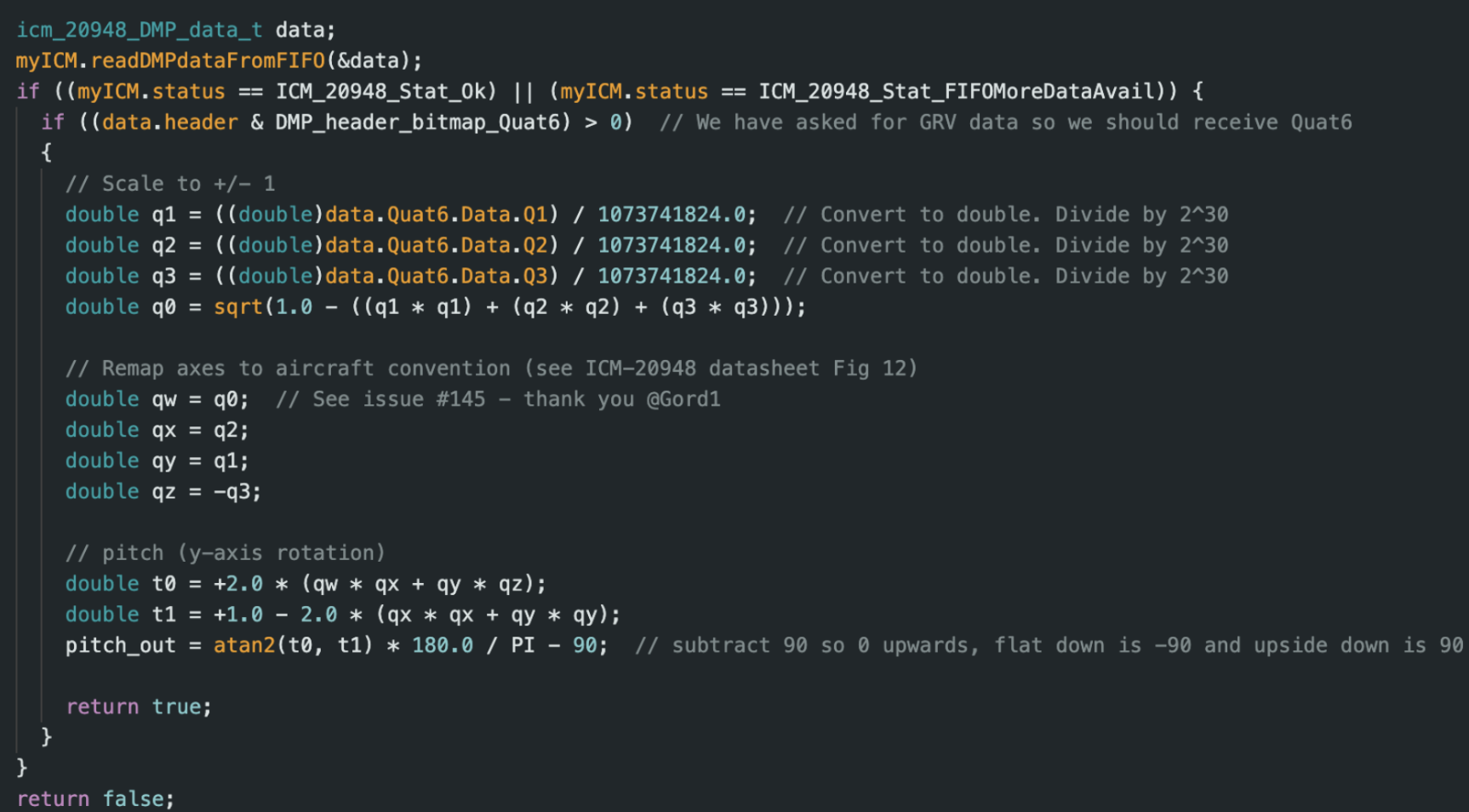
DMP Calculation
I gather the DMP data like previous labs but get the pitch instead. I subtract 90 so it matches the reference pitch in Figure 2.
Raw Gyro Calculation
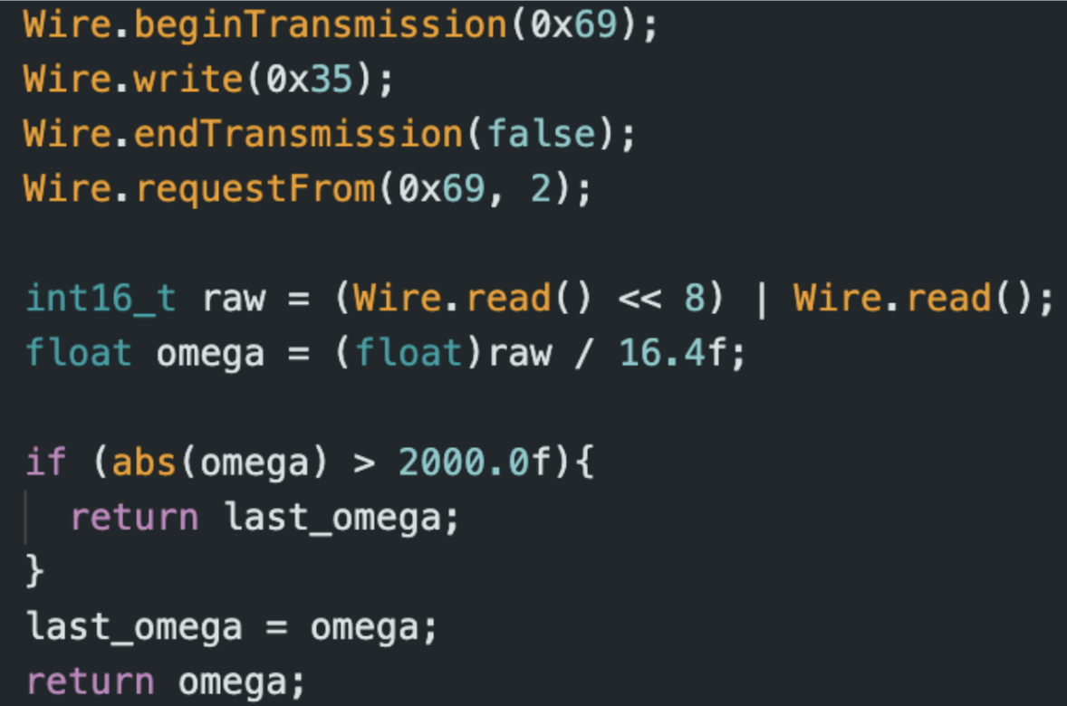
The IMU’s address is 0x69, and we start communication/begin to queue up a transmission. We want to first tell the sensor which register we want to read the information from and then read the appropriate bytes. We do “Wire.write(0x35)” to have the register pointer point to this address because of Figure 3 below. AGB0_REG_GYRO_YOUT_H is 0x35, and AGB0_REG_GYRO_YOUT_L is 0x36. Then I do Wire.endTransmission(false) so that the I²C bus isn’t released yet (don’t want TOF intercepting). Then I request 2 bytes from the IMU (which will be the high and low bytes of the gyro’s Y direction). This request makes the MCU the receiver now. We first read the high byte and shift it over 8 bits, and then we read the low byte. These two bytes are then bitwise ORed to get a raw gyro value in the Y direction from -32,768 to 32,767 since it is signed. This is the raw value and must be converted to usable units in deg/s. Since the DMP puts the IMU in +/-2000dps mode. Referencing the datasheet for this sensor, this mode corresponds with a scale factor of 16.4, so our angular velocity in deg/s is the raw value divided by 16.4. Also, since we are in the +/-2000 dps mode, we do a simple check to see if the absolute value of the measurement is greater than 2000 and, if so, reject it and use the old value.
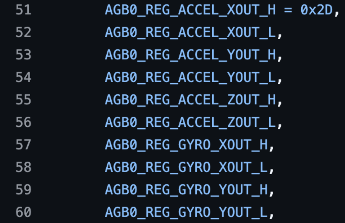
Figure 3. Register list from ICM_20948_REGISTERS.h.
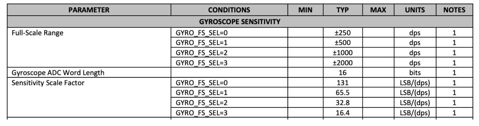
Figure 4. Table for the gyro settings from the datasheet.
Controller techniques
P term
I made Kp large since we want to shoot up to the set point once we get airtime. I was thinking of having dynamic gain values that depend on a range of pitch values, but was too difficult to tune.

I term
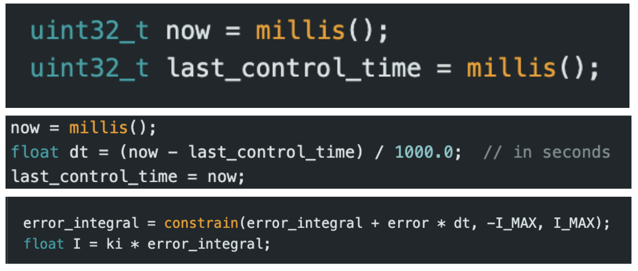
The I term uses a dynamic dt, so I calculated the time between each loop iteration with the millis() function and converted it to seconds so the gain parameters are easier to work with. To prevent integrator windup, I had a maximum value of 920, which is the max PWM times 4 for more granularity (KI gain will be smaller).
D term
I have an “omega_deadzone” variable (omega is angular velocity). If omega is within -40.5 to 40.5deg/s, then I set it to 0; otherwise, I keep the value. This is to avoid the noise at lower zones for less jitter when it is near its set point. I got this value from rotating the robot with my hand and picking a speed that I thought was fast enough for the D term to be necessary. Of course there is still noise at higher speeds, so I implemented a low-pass filter to deal with noise at higher frequencies. My tuned alpha is 0.5. The derivative term is clamped at 200 PWM, so it doesn’t dominate the controller.
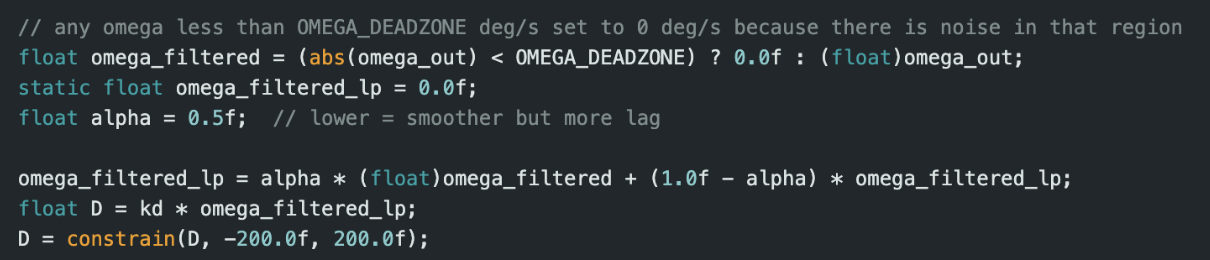
Deadband
Huge shoutout to Jack Long for this idea! Basically, without a dead band, my controller would always be outputting some PWM value even when the robot is perfectly balanced. This leads to a very jittery robot. To fix this, if the error is between -1.67 and 1.67 degrees, the motors will turn off, and we reset the “integral_error” to prevent windup. Before it would jitter like crazy and make itself even more unstable.
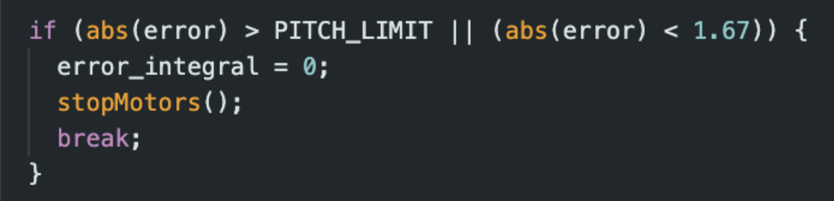
Pitch limit
If the robot is within “PITCH_LIMIT=80” degrees from the set point in either direction, the controller will activate; if not, the controller will deactivate and brake. It's high because I wanted to initiate the controller early during the flip. I didn’t want the flip to be too aggressive because then it would be harder to control. 80 degrees is technically inaccurate because I am using a linear controller on a nonlinear system (you can only approximate this system as linear at small angles), but it is ok because the controller will shoot up fast, and then the derivative term will slow it down so that the system enters the linear regime quickly.
Debugging
I printed out each P, I, and D term and analyzed their relative weights to see how I should tune my gain. My final values were Kp=14.2,Ki=0.3,Kd=0.36.
PID Output
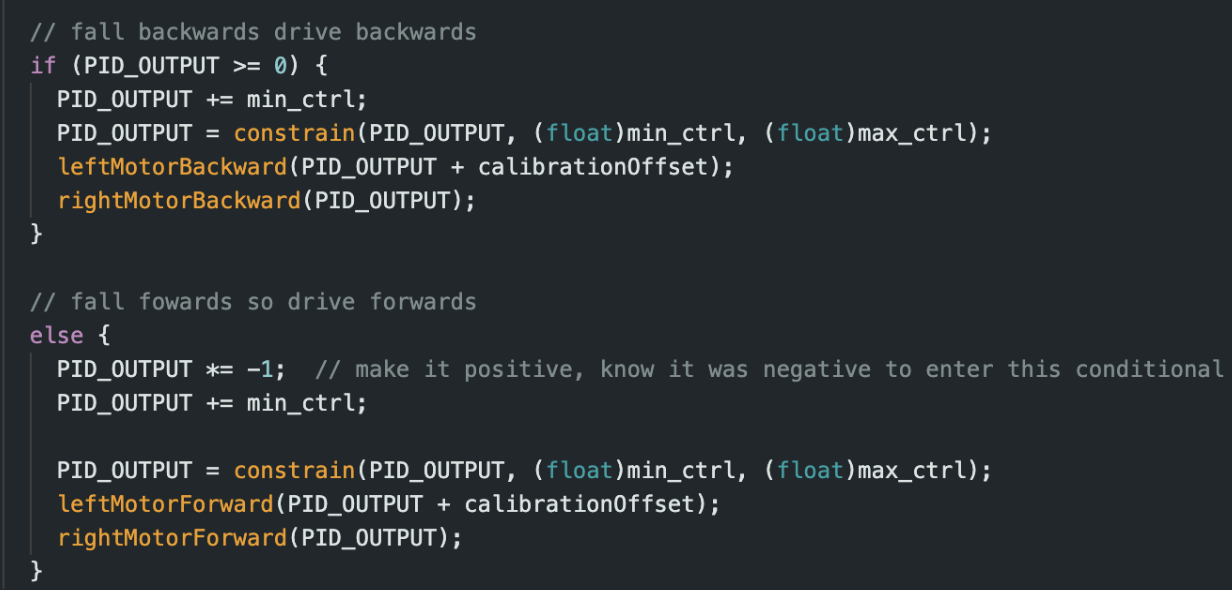
As seen in figure 1, the D term is negative, so PID_OUTPUT=P-D+I. If the robot falls forwards, we drive forwards, or if it falls backwards, we drive backwards to self-right ourselves. If PID_OUTPUT>=0, this means set_point>measured pitch, so we are falling backward, so we must drive backward. We always add min_ctrl so we have more granularity for my controller. Min_ctrl isn’t enough to move the robot but gets the PWM higher so there is less dead space.
The Flip
I could not consistently get it to flip at first, so I focused on balancing it with me pushing it up for Robot Day. Before, I tried driving forwards and then immediately backwards. I even tried driving the robot back and forth multiple times. I also tried running into a wall and then balancing.
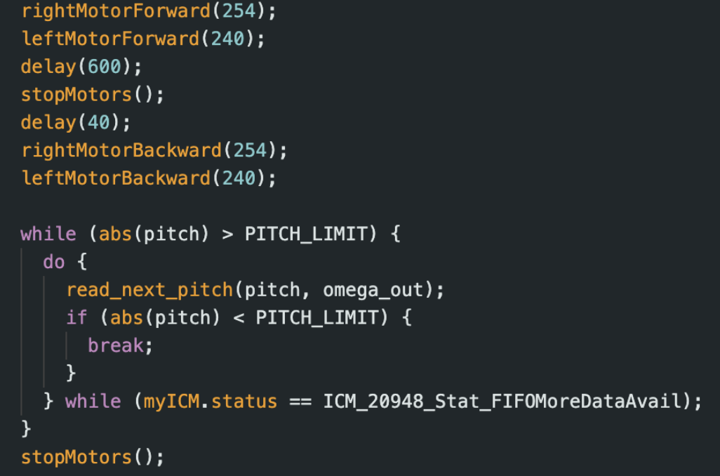
After Robot Day, I used the flip mat and was successful. My final sequence was to drive the robot forwards at full speed for 600 ms, break briefly for 40 ms, and then continuously drive backwards until I received a pitch value within the PITCH_LIMIT, and then I activated my controller.
Slight Change in Setpoint
The angular momentum from the flip carries the robot forward, so I have the set point as -5 degrees initially to bring it back, and then the set point goes back to -0.7°.
Favorite Video
Other Successful Videos
My controller is reliable and can last for a few seconds. Usually anywhere from 3-9 seconds without hitting a wall.
Progress for planning & execution lab
I used a TOF sensor as a motor encoder but didn’t do the other lab option. I was going to use it as odometry data for the prediction step of the Bayes filter. The granularity is half the wheel’s circumference (255/2=127.5mm), which would've been great since the granularity of the grids is 304.8mmx304.8mm.
Collaborations
Thank you, Professor Helbling. I referenced Nita Kattimani’s site. Jack Long suggested deadband. Hunter inspired this website and the PID control diagram. An LLM was used to help me think about direct register reading. One of my favorite classes at Cornell!