Lab
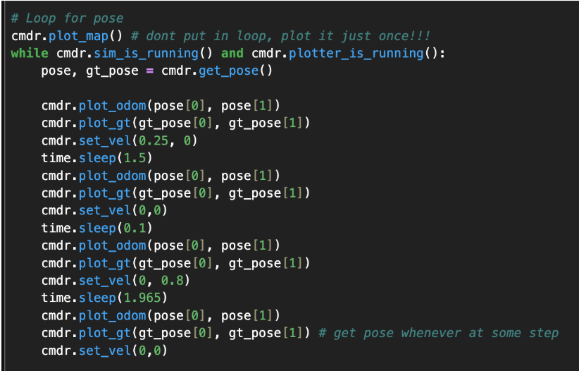
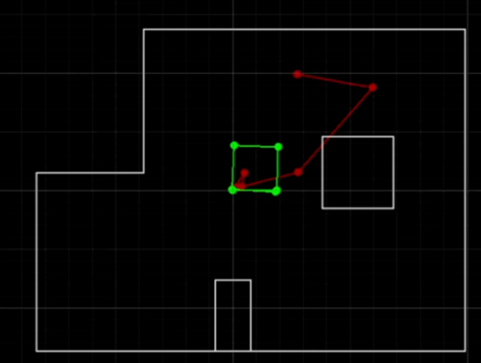
Nonprobabilistic methods like odometry lead to poor results, as seen in the prelab.
compute_control
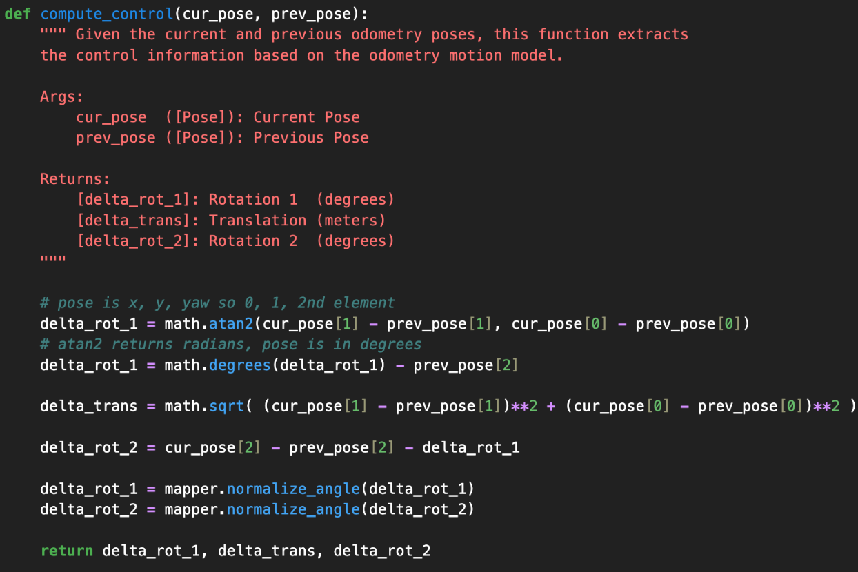
I followed the odometry model theory discussed in class:
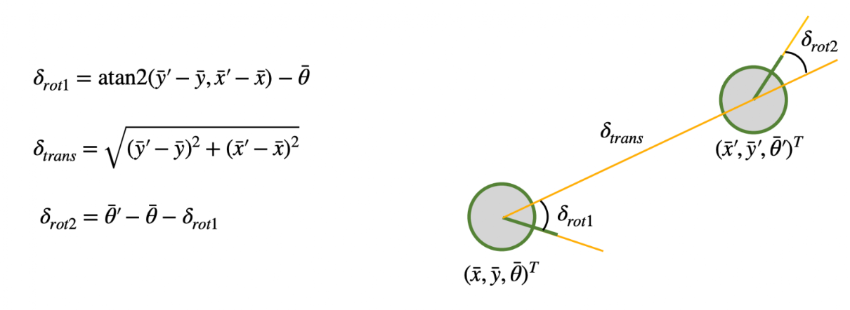
Delta_rot_1 will orient the robot initially, then delta_trans will bring the robot to its final xy position, and then delta_rot_2 rotates the robot again to get the robot's final orientation.
odom_motion_model
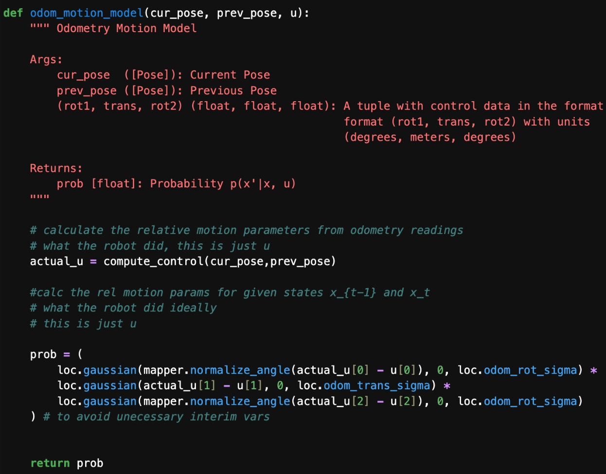
I followed the algorithm from class.
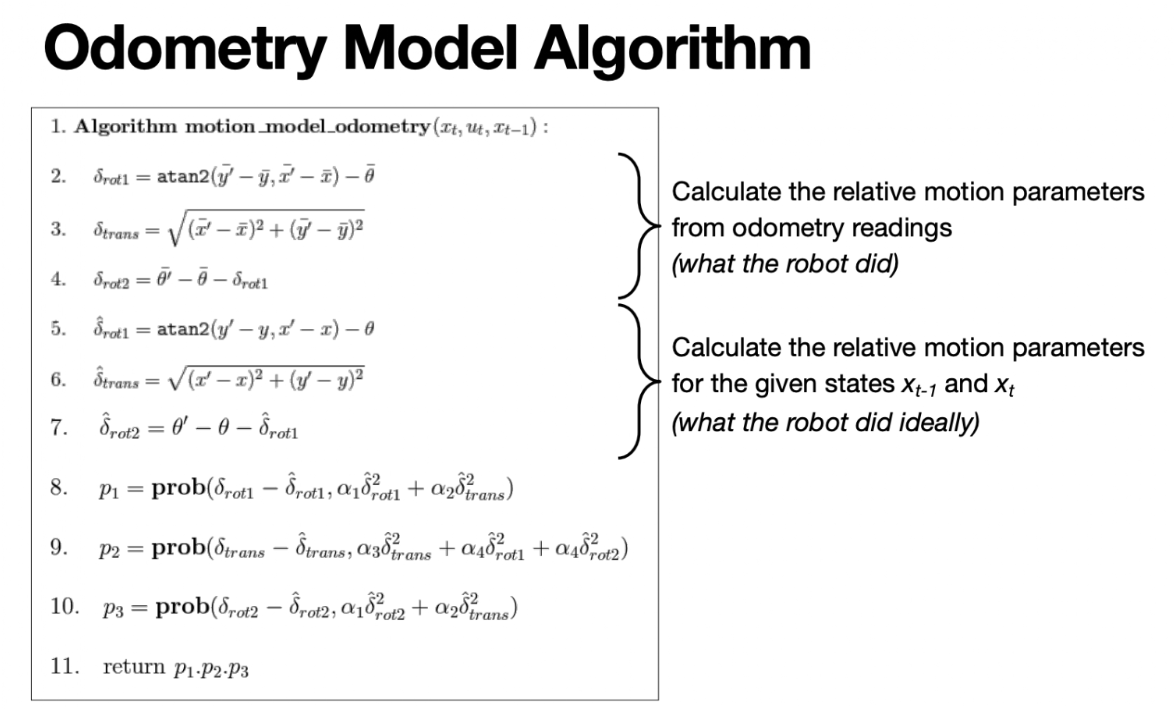
I made sure to normalize the angle again. "Actual_u," which is computed using compute_control(cur_pose,prev_pose), is what the robot did, and "u" is what the robot did ideally. We then substitute these parameters into a Gaussian to find the likelihood of the robot going from its prev_pose to cur_pose given that the current control action is "actual_u." This probability p(x’|x,u) is calculated by this function, and we multiply the three known probabilities, as they are independent.
prediction_step

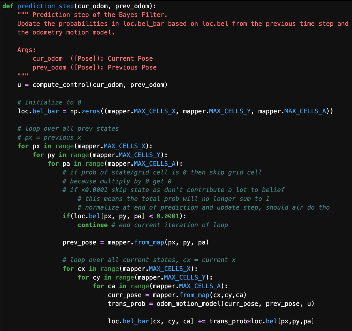
Here we loop through all the possible states/grid cells in the 12x9x18 space and get the previous and current states of each grid cell. We optimize by skipping grid cells with a bel/probability that is <0.0001, as it will practically multiply to 0. Of course, not all the time will it be exactly 0, so our probability no longer adds up to 1, but we will normalize in our update step as we would do anyway.
update_step with sensor_model
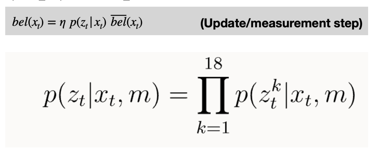
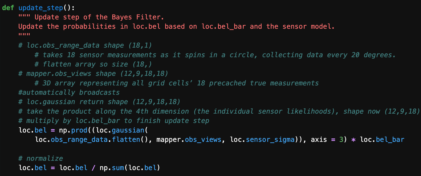
We don’t use the sensor_model helper function and instead do those calculations in update_step so we can vectorize for efficiency. Conceptually, we have “mapper.obs_views” as our mean since it is the true observation/the sensor should read at that grid cell in the map. Given this true observation, we are calculating how likely the noisy sensor measurement is (obs_range_data.flatten); of course, we assume the sensor noise is Gaussian with an SD of loc.sensor_sigma. To deal with floating-point underflow, we normalize the belief at the end. However, we were supposed to normalize anyway because we multiply by η.
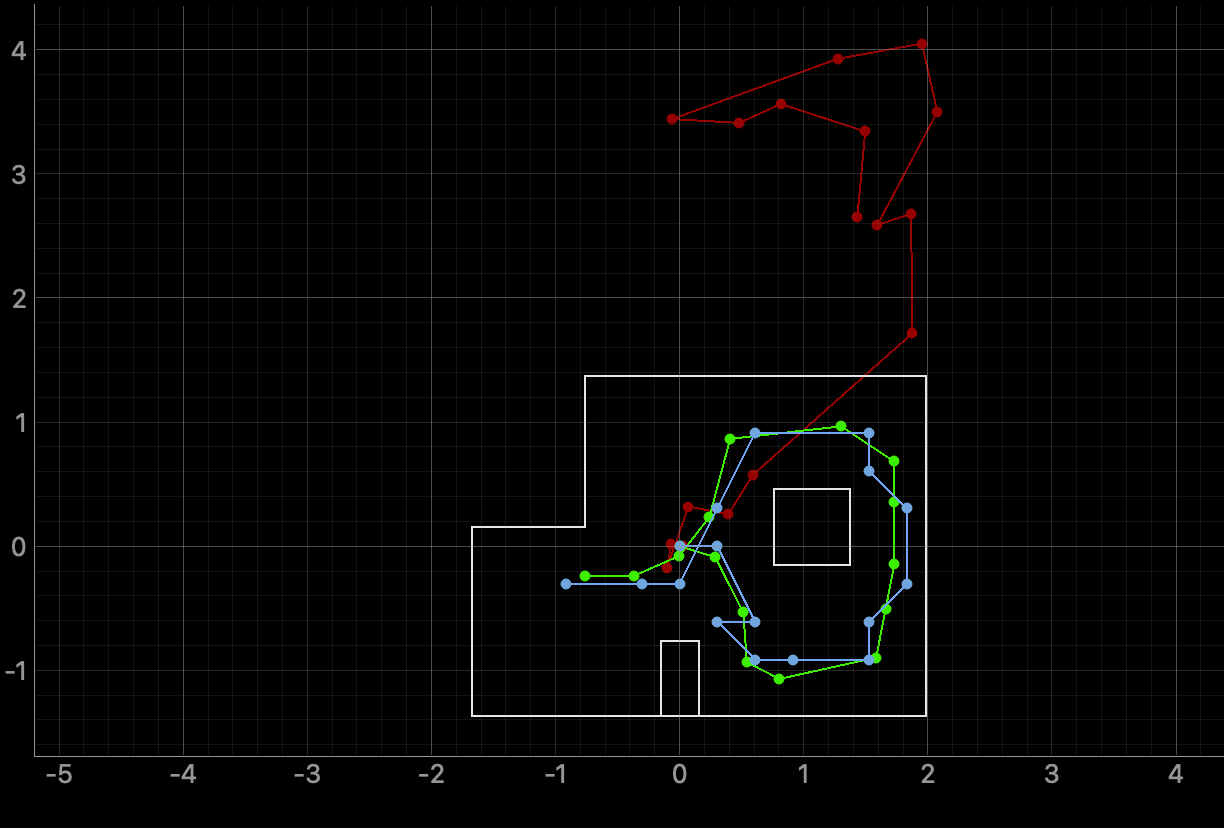
Run 1
Run 2
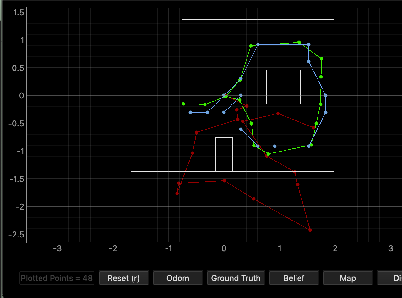
The most probable state is “bel index,” and it gives its probability, and the ground truth is "GT." For run2, it works well at steps 3,5,13,14. For example, step 3 has a ground truth of x=0.542m and y=-0.933m and a belief of x=0.610m and y=-0.914m–very minimal error. I struggle at steps 2, 7, and 10 the most for the latest run. For step 2, the error is 0.209m for the x direction, and the bel_bar is 4.6e-37≈0. The prediction step is uncertain here. It works well when the bel_bar is reasonably high, as that means the prediction got to roughly the right area, and the update sensor step just raises the likelihood of it being there. When the robot is near corners/walls, this allows the update step to be more confident as the sensor has more unique and useful data to correct the prediction step. If bel_bar≈0, then the prediction step is practically useless, and we have to rely on the sensor. Since our sensor has noise, it doesn’t give the best location. Angle errors are frequent and common because it is harder to distinguish between orientations that look similar sensor-wise. Also, large steps in distance are an issue since odometry/motion models only work well for short distances. Regardless, the blue (Bayes output) is much closer to the green (ground truth) than the red odometry, as expected.
Collaborations
Thank you Prof. Helbling. I referenced Aidan McNay's, Stephan Wagner's, Aidan Derocher's, and Jonathan Ma's websites. Hunter inspired this website template.